Assessing riparian vegetation structure and the influence of
land use using landscape metrics and geostatistical tools
Maria do Rosário Pereira Fernandes
Dissertação para obtenção do grau de Mestre em
Engenharia Florestal e dos Recursos Naturais
Orientador: Maria Teresa Ferreira da Cunha Cardoso
Júri:
Presidente: Doutor José Miguel Oliveira Cardoso Pereira, Professor Catedrático do Instituto Superior de Agronomia da Universidade Técnica de Lisboa Vogais: Doutora Maria Teresa Marques Ferreira da Cunha Cardoso, Professora
Associada do Instituto Superior de Agronomia da Universidade Técnica de Lisboa; Doutor José Guilherme Martins Dias Calvão Borges, Professor Associado do
À Profª Maria Teresa Ferreira pela orientação científica, amizade, motivação e toda a
confiança depositada.
À Doutora Francisca Aguiar pela revisão detalhada de todo o manuscrito, pela amizade e por
todos os valiosos conselhos pessoais e profissionais.
Ao Doutor Pedro Segurado pelas sugestões e leituras e ao Mestre Paulo Branco pela
correcção e crítica do artigo.
À Profª Cristina Catita pelo incentivo e esclarecimentos prestados.
A todos os colegas do “Waterlobby” pela amizade, disponibilidade e companheirismo.
Aos meus pais pelo apoio incondicional e pelo carinho permanente.
métricas de paisagem e geoestatística
Resumo
O objectivo do estudo é a avaliação da adequação de métricas de paisagem na descrição e caracterização da estrutura ripária e da sua resposta à influência dos usos do solo proximais (30m) e distais (200m). A área de estudo localizou-se na bacia hidrográfica do Tejo tendo sido cartografada a vegetação ripária de quatro ribeiras, classificada nas componentes arbórea, arbustiva e herbácea. Oito métricas de paisagem relacionadas com configuração espacial, isolamento, distribuição e inter conectividade foram calculadas para os três estratos de vegetação. A influencia dos usos do solo na estrutura da vegetação foi avaliada por análise de redundância e a componente espacial dos dados biológicos foi incorporada utilizando métodos de geoestatística.
Os resultados demonstram que a combinação de métricas de diferentes categorias funcionais permite descrever de forma eficiente a estrutura da vegetação ripária, sobretudo ao nível da classe arbórea. A inclusão de unidades de amostragem espacialmente independentes aumentou drasticamente a variabilidade explicada pelos usos dos solo, em particular o uso proximal, que de forma consistente apresentou maior influência na estrutura da vegetação ripária. Em situação de elevada pressão, nomeadamente em zonas agrícolas, a vegetação ripária apresentou padrões de fragmentação caracterizados por um número reduzido de pequenas manchas de vegetação lenhosa, relativamente homogéneas com configurações simples e reduzida conectividade.
Palavras chave: Galerias ribeirinhas, pressões antropogénicas, métricas espaciais,
using landscape metrics and geostatistical tools
Abstract
The present work aims to identify potential landscape metrics that best describe and quantify the riparian structure and evaluate its response to land use pressure. The study was conducted in four rivers of the Tagus fluvial system Data was achieved from the on-screen photo interpretation of airborne digital images. Eight landscape metrics related with the spatial configuration, isolation, inter-connectivity and distribution of riparian vegetation were calculated for the tree, shrub and herbaceous strata. The influence of proximal and distal land use (30 m and 200 m buffers, respectively) in the riparian structure was analysed using redundancy analysis. Geostatistical analysis were used to describe and incorporate the spatial component of the data and to assess the spatial autocorrelation of the riparian structure. The results showed that the combined interpretation of metric values can consistently describe the patterns of riparian structure especially for the tree cover class. Disturbed riparian woods due to major land use pressure, such as agriculture, presented a low number of small patches with simple and homogenous shapes, reduced patch connectivity and a non interspersed patch distribution. Also it is shown that the proximal land use is more determinant in shaping within-stand riparian structure, therefore protection areas should both envelop riparian zones and an adjacent buffer.
Resumo alargado
O avanço das técnicas de avaliação remota e das tecnologias SIG (Sistemas de Informação Geográfica) abriram novas perspectivas quer no campo da análise descritiva da vegetação, quer no âmbito da ciência aplicada, possibilitando o desenvolvimento de ferramentas de apoio à gestão de áreas fluviais, incluindo zonas ripárias. Como exemplo, refira-se a importância destas tecnologias na implementação de Directivas Comunitárias como a Directiva Habitats (92/43/EEC; European Council, 1992), e a Directiva Quadro da Água (EU/2000/60; European Council, 2000). No entanto, poucos trabalhos fazem uso destas técnicas, nomeadamente no que se refere à descrição e caracterização da vegetação ripária e ao seu uso como bioindicador da qualidade ecológica fluvial. A estrutura e integridade da vegetação ribeirinha encontram-se ainda pouco esclarecidas, sobretudo em sistemas mediterrânicos sujeitos a perturbações milenares no uso do solo das zonas adjacentes aos sistemas fluviais (Stromberg, 1993; Corbacho et al., 2003;von Schiller et al., 2008).
O ponto de partida deste trabalho baseia-se na premissa de que padrões espaciais de reduzida conectividade e elevados níveis de fragmentação na vegetação ribeirinha traduzem uma reduzida condição fluvial (Petersen, 1992; Schuft et al., 1999), sendo preditivos do nível de intervenção humana sobre o sistema (Johansen et al., 2007). É ainda consensual que o uso do solo influencia a estrutura da vegetação ripária, sendo responsável pela redução da sua integridade (Aguiar et al., 2005). Alguns trabalhos (e.g. Bunn and Davies, 2000; Bott et al., 2006) sugerem uma maior influência na estrutura da vegetação ripícola do uso do solo próximo da galeria ribeirinha, em relação ao das zonas mais afastadas.
usos do solo proximais e distais, testados neste caso, em buffers de 30m e 200m, respectivamente.
O trabalho teve início com a cartografia da vegetação ripária, dividida na componente arbórea, arbustiva e herbácea, realizada por fotointerpretação sobre ortofotomapas digitais (RGB, 0,5 x 0,5 m por pixel, cobertura na Primavera de 2005) em quatro ribeiras pertencentes à bacia hidrográfica do Tejo. De seguida, oito métricas de paisagem (Number of Patches (NP), Mean Patch Size (MPS), Patch Size Coefficient of Variation (PSCV), Mean Shape Index (MSI), Mean Fractal Dimension Index (MPFD), Mean Nearest-Neighbor Distance (MNN), Mean Proximity Index (MPI) e Interspersion and Juxtaposition Index (IJI) foram calculadas, aplicadas às três classes de vegetação, recorrendo à extensão Patch Analyst- vector format para ArcGIS 9. A avaliação da influência dos usos do solo na estrutura da vegetação foi realizada com recurso a análise multivariada (análise de redundância). Técnicas de análise espacial, nomeadamente a função variograma e o Índice de Moran (Moran, 1950), foram utilizadas para estimar e incorporar a componente espacial dos dados biológicos e para avaliar o nível de dependência espacial (autocorrelação) da estrutura da vegetação ripária. Os resultados demonstraram que a combinação de métricas de diferentes categorias funcionais, permitem descrever de forma eficiente a estrutura da vegetação ripária, sobretudo quando aplicadas ao nível de classe arbórea. Como exemplo, apontam-se as manchas de vegetação encontradas em zonas de baixa perturbação humana que evidenciam, de forma constante, padrões de elevada conectividade e complexidade geométrica, e manchas de vegetação herbácea com configurações simples e alongadas associadas a zonas de maior actividade agrícola. Os padrões espaciais de distribuição da vegetação ripária apresentaram variações ao longo do gradiente existente de crescente influência antropogénica
(agro-vegetação ripícola lenhosa. A estrutura da (agro-vegetação ripária apresentou dependência espacial, com comportamentos locais acentuados, sobretudo na classe arbórea. A utilização de unidades ripárias de amostragem espacialmente independentes permitiu aumentar, significativamente, a variabilidade explicada pelos usos do solo na estrutura ripária. Em situação de dependência espacial a complexidade estrutural da vegetação é devida sobretudo à sua componente espacial, e não à influência dos usos do solo.
Face à resposta das métricas ao uso do solo é possível descrever uma paisagem ripária em situação de degradação, sobretudo no que se refere a alterações derivadas do uso intensivo do solo para a agricultura. Nestas condições, a galeria ribeirinha será caracterizada por um número reduzido de pequenas manchas de vegetação lenhosa (valores reduzidos para as métricas NP e MPS). Ocorrerá uma homogeneização no tamanho das manchas de vegetação (valores reduzidos de PSCV) o que implicará perda da variabilidade natural intraespecífica. A vegetação lenhosa apresentará reduzida conectividade (valores reduzidos de MPI) com padrões de fragmentação caracterizados por um acentuado afastamento entre as manchas de vegetação ripária lenhosa (elevados valores de MNN) e uma distribuição desequilibrada dos diversos estratos ao longo da galeria ribeirinha (valores reduzidos de IJI). Em relação à forma das manchas espera-se que estas tendam a apresentar uma maior simplicidade, perdendo as configurações meandrizadas e intrincadas observadas nas zonas com menor intervenção humana (valores reduzidos de MSI e de MPFD).
O trabalho sugere uma metodologia inovadora e eficiente para caracterização da estrutura da vegetação ripária funcionando como uma ferramenta útil na gestão e conservação das zonas ribeirinhas uma vez que permite identificar zonas prioritárias de reposição dos padrões de conectividade e redução dos níveis de fragmentação.
Índice
Índice de Tabelas... 2
Índice de Figuras... 3
Artigo: Assessing riparian vegetation structure and the influence of land use
using landscape metrics and geostatistical tools...
4
Abstract... 5
1. Introduction... 7
2. Methodology... 10
2.1 Study area
...
10
2.2 Riparian vegetation structure and land use assessment
...
10
2.3 Spatial autocorrelation assessment
...
12
2.4 Influence of land use in the riparian vegetation structure
...
14
3. Results... 16
3.1 Riparian structure
...
16
3.2 Spatial autocorrelation
...
17
3.3 Land use and spatial influence in the riparian vegetation structure
...
18
3.4 Influence of land use variables in tree cover class
...
19
4. Discussion... 20
4.1 Assessing riparian structure through landscape metrics
...
20
4.2 Spatial autocorrelation assessment
...
21
4.3 Influence of land use in the riparian vegetation structure
...
22
5. Conclusion and implications for riparian management... 24
Índice de Tabelas
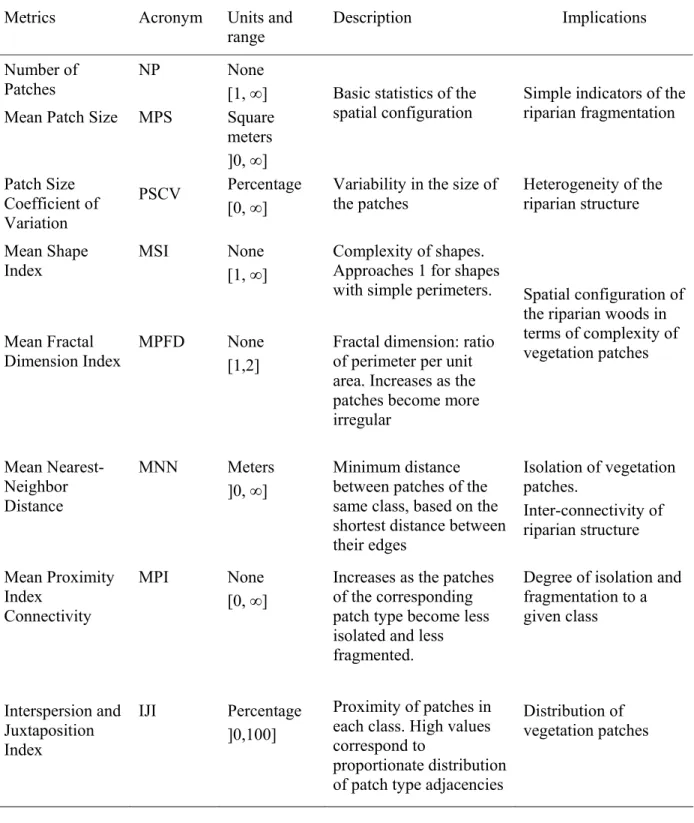
Table 1. Metrics, acronyms, units, range, description (formulae and detailed calculation from McGarigal and Marks, 1994) and implications in the characterization of riparian vegetation structure………..32
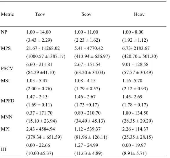
Table 2. Minimum and maximum values, average ± SD (in parentheses) for the tree, shrub and herbaceous cover classes per Sampling Unit. Metric acronyms are given in Table 1. Cover classes: Tcov- tree, Scov – shrub, Hcov-herbaceous………...33
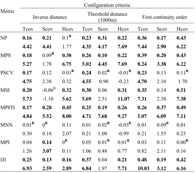
Table 3. Moran’s I and z-scores for the riparian metrics, using different configurations of the spatial proximity matrix. Significant cluster patterns are indicated in bold, random patterns are indicated as R (**P<0.01). Metric acronyms are given in Table1. Cover classes: Tcov- tree, Scov – shrub, Hcov-herbaceous………..………...34
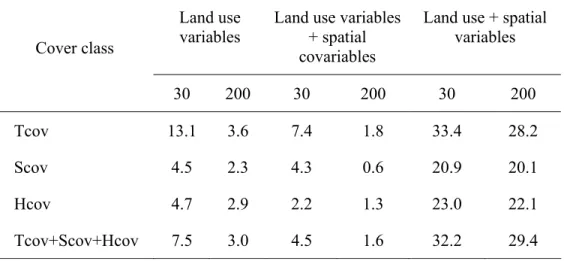
Table 4. Contribution to total variance (%) of explanatory variables using RDA with solely land use variables, land use variables and spatial co-variables and land use and spatial variables, per vegetation class (n=330) with the 30 and 200 m buffers. Cover classes: Tcov- tree, Scov – shrub, Hcov-herbaceous……….35
Table 5. Minimum and maximum values, average ± SD (in parentheses) of the contribution to total variance (%) of land use variables per cover class, using non-autocorrelated SU (9 combinations, n=28) in 30 and 200 m buffers. Cover classes: Tcov- tree, Scov – shrub, Hcov-herbaceous………..36
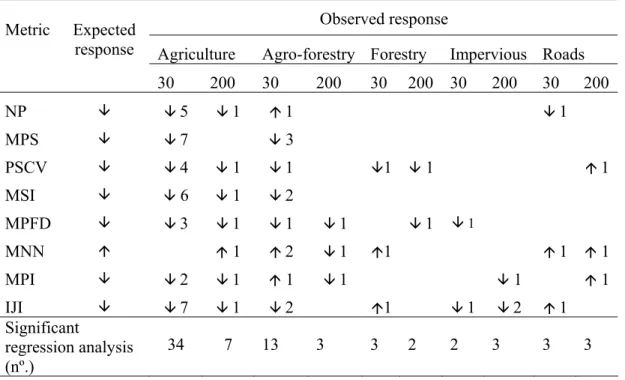
Table 6. Expected and observed responses to land use increase (Ç - positive relation, È - negative relation) and number of significant multiple regression analysis (*P<0.05) in the 30 and 200 m buffers. Metric acronyms are given in Table 1……….37
Índice de Figuras
Figure 1. Iberian Peninsula, showing the Portuguese part of the Tagus basin and the location of the four river basins……….…39
Figure 2. Semivariogram function (adapted from Main et al., 2004)……….…………40
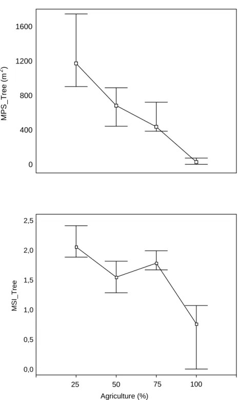
Figure 3. Median, 25 and 75 quartile for the Mean Patch Size (MPS) and Mean Shape Index (MSI) of the tree cover class with the increase of the agricultural areas in the 30 m buffer (n=28 SU, 9 combinations)………..41
Assessing riparian vegetation structure and the influence of land
use using landscape metrics and geostatistical tools
(Submitted to Forest Ecology and Management)
Maria Rosário Fernandes, Francisca C. Aguiar and M. Teresa Ferreira
Centro de Estudos Florestais, Departamento de Engenharia Florestal, Instituto Superior de Agronomia, Tapada da Ajuda, 1349-017, Lisboa, Portugal
*Author for correspondence (email: [email protected]; phone: +351 213653487; fax: +351 213645000)
Abstract
Mapping riparian structural attributes in a fine scale resolution can provide useful information for the management, conservation and restoration of streams. The present work aims to identify potential landscape metrics that best describe and quantify the riparian structure and evaluate its response to land use pressure.
The study was conducted in four rivers of the Tagus fluvial system (Portugal). Data was achieved from the on-screen photo interpretation of airborne digital images (RGB-NIR spatial resolution 0.5 x 0.5 m, spring 2005). River stretches were divided in Sampling Units of 250 meters long, and patches of riparian woody vegetation (tree, shrub and herbaceous strata) were delineated. Eight landscape metrics, namely Number of Patches (NP), Mean Patch Size (MPS), Patch Size Coefficient of Variation (PSCV), Mean Shape Index (MSI), Mean Fractal Dimension Index (MPFD), Mean Nearest-Neighbor Distance (MNN), Mean Proximity Index (MPI) and Interspersion and Juxtaposition Index (IJI), related with the spatial configuration, isolation, inter-connectivity and distribution of riparian vegetation were calculated for all strata. The influence of proximal and distal land use (30 m and 200 m buffers, respectively) in the riparian structure was analysed using redundancy analysis. Geostatistical analysis (semivariogram, global and local Moran´s I) were used to describe and incorporate the spatial component of the data and to assess the spatial autocorrelation of the riparian structure. The results showed that the combined interpretation of metric values can consistently describe the patterns of riparian structure especially for the tree cover class. The inclusion of spatial independent sample units increases drastically the contribution of the land use variables to the total explained variance of the riparian structure. Disturbed riparian woods due to major land use pressure, such as agriculture, presented a low number of small patches (low NP and MPS values) with simple and homogenous shapes (low MSI, MPFD and PSCV values), reduced
patch connectivity (high MNN values and low MPI values), and a non interspersed patch distribution (low IJI values). Also it is shown that the proximal land use is more determinant in shaping within-stand riparian structure, therefore protection areas should both envelop riparian zones and an adjacent buffer.
1. Introduction
Riparian zones are responsible for many ecological functions considered crucial for the preservation of river ecological conditions (Forman, 1997; Naiman and Décamps, 1997). Stream management and restoration programs such as the European Union’s Water Framework Directive (EU/2000/60; European Council, 2000), have broadly recognized the urgent need of developing methodologies to evaluate ecological river quality. Some studies focused the floristic composition (e.g. Looy et al., 2008), structural and functional attributes, like longitudinal and lateral continuity of woody vegetation, natural woody regeneration (e.g. González-del-Tánago and García-Jalón, 2006), percentage of canopy cover, canopy continuity, tree clearing (e.g. Johansen and Phinn, 2006), but all require intensive field survey. Other methods are expedite and visually based but involve no quantification (e.g. Ward et al., 2003; Dixon et al., 2006). In other cases, using remotely sensed image data, the riparian zone is considered a fixed buffer (e.g. Schuft et al., 1999; Congalton et al., 2002; Yang, 2007) and the mismatch between the riparian buffer and the really existent riparian zone might cause errors in the estimation of vegetation cover. Thus, efficient and quantitative remote measurements of riparian vegetation would be useful, especially if they could relate in some way to riparian quality and human influence upon it. However, image based methods (satellite images or airborne digital images) become increasingly more cost-effective than field assessments, when a higher level of detail is necessary (Johansen and Phinn, 2006). Moreover, high spatial resolution imagery (< 5 x 5 m pixels) is essential for mapping riparian vegetation due to the limited width of riparian zones and the high spatial variability (Muller, 1997; Congalton et al., 2002; Davis et al., 2002).
Resourceful tools, such as landscape metrics, derived with Geographical Information System techniques, can characterize the structural attributes of woody vegetation (Apan et al., 2002).
Landscape metrics are numeric descriptors of spatial configuration, such as density, distribution, complexity, isolation, dispersion contagion and interspersion. Description and quantification of riparian vegetation using landscapes metrics improves the awareness of riparian structural-functional associations, since spatial patterns can influence ecological processes affected by riparian patch configuration, connectivity and distribution (Rex and Malanson, 1990; Turner, 1989). Reduced connectivity and fragmented patterns, particularly in the woody vegetation, represent lower stream ecological conditions (Schuft et al., 1999). Also, the vegetation structure of riparian zones can reveal the level of human disturbance and can be used as an environmental indicator of riparian zone condition (Johansen et al., 2007). In this study, riparian structure is defined as the longitudinal continuity of the riparian vegetation patches, its aggregation, configuration, expansion limits and distribution in the riparian zone.
Land use influences the composition and integrity patterns of riparian vegetation (Décamps et al., 1988) and other structural attributes at different scales (Allan, 2004) especially in Mediterranean riparian landscapes (Stromberg, 1993; Corbacho et al., 2003; von Schiller et al., 2008). The proximal and distal land use has been suggested to influence differently the stream functions (Bunn and Davies, 2000; Bott et al., 2006) and the riparian structure (Aguiar et al., 2005). The traditional statistical approaches to study the influence of environmental in the vegetation are based in the assumption of randomness and therefore in the independence of the sample (Miller et al., 2007). This violates one of the basic principles of Geography and Ecology, the direct relationship between proximity and similarity (Tobler, 1979). However, the closely elements in an ecosystem tend to be influenced by the same processes and have a propensity to present higher likeness (Legendre and Fortin, 1989); a phenomenon called Spatial Autocorrelation. This fact introduces the spatial component into the ecological analysis and should not be ignored; otherwise it can lead to erroneous results.
Taken into account the spatial component of the data, the present study aims to: 1) assess the ability to describe the riparian vegetation structure using landscape metrics, 2) identify the land uses that significantly influence the structure of the riparian vegetation, and 3) evaluate the magnitude of the influence of proximal and distal land use using riparian landscape metrics.
2. Methodology
2.1 Study area
The study was conducted at four rivers of the left margin of River Tagus (Chouto, Margem, Muge and Sôr) (Figure 1), with similar climate and geomorphology. The studied stretches are mostly spread over calcareous Mesozoic formations and have a Mediterranean climate, with a high seasonal variability of rainfall patterns. According to the Atlas do Ambiente
(http://www.iambiente.pt/atlas/), the annual runoff ranges from 200 a 300 mm, with an annual
average rainfall of 600 a 800 mm and an annual average temperature of 15-17.5 oC. The land use in the study area is very heterogeneous with small-scale agriculture (e.g. orchards, vineyards, maize), pine and eucalyptus forests, mediterranean shrublands, cork oaklands, interrupted by few and low-populated human settlements. In general, the riparian woods are narrow, frequently with less than 10 meters width and are dominated by ashes (Fraxinus angustifolia), alders (Alnus glutinosa) and Salix species; the shrub strata include species like the hawthorn (Crataegus monogyna), the black-elder (Sambucus nigra) and the alder buckthorn (Frangula alnus) (Aguiar et al., 2000).
2.2 Riparian vegetation structure and land use assessment
A Geographic Information System was used to store and organize the data achieved from the on-screen photo interpretation of 1:5000 airborne digital images (RGB-NIR spatial resolution 0.5 x 0.5 m; ortho-rectified and mosaicked, flyover date spring 2005) and to calculate the metrics of the riparian vegetation structure.
First, the river stretches were divided in 250 m long sampling units (SU) and the limits of the riparian vegetation were manually defined in both banks. Then, the riparian vegetation
patches were classified in trees, shrubs and herbaceous vegetation and mapped within each SU using visual screening of textural image features (color, grain). Patches with shadow, water and bare soil were not considered. Finally, eight landscape metrics calculated with the Patch Analyst – Vector format (ArcGis9) extension were used to describe the riparian vegetation, in terms of spatial configuration, isolation, inter-connectivity and distribution (Table 1).
A connectivity distance of five meters was applied to the MPI calculation, as used by Schuft et al. (1999) in the characterization of riparian-stream networks.
Kolmogorov-Smirnov test and the Spearman rank correlation (R) were used to evaluate the normality and the relations between metrics, respectively. The correlated metrics (|
R|
> 0.8) were eliminated to avoid redundancy in the data.Two buffers contiguous to the fluvial corridor, 30 m and 200 m were defined to evaluate the influence of proximal and distal land use in the riparian vegetation structure, respectively. A previous assessment of the existing land uses was made using fifty SU scattered in the study area. Four land use classes were defined and considered as positioned along the following increasing gradient of anthropogenic pressure: 1) agro-forests (extensive crops, pastures, scrubland, oak and cork-oak woodlands, fallow ground and mixed woodland, 2) forest (plantations of pine and eucalyptus), 3) agriculture (irrigation crops, rice fields, orchards and vineyards), 4) impervious (urban and industrial areas). Land use classes were evaluated in percentage of area occupied per buffer, after grouping the various patches within each SU. Roads were also taken into account and quantified in length (km) per SU and per buffer.
Field observations were made during the summer season of 2007 to calibrate and validate the photo interpretation.
2.3 Spatial autocorrelation assessment
Studies on the distribution of biological data or ecological variables display a certain degree of spatial dependence, usually termed as spatial autocorrelation (SAC), a measure of similarity of an attribute within an area (Anselin, 2002). SAC measures the correlation of a variable with itself through space, i.e the lack of independence between pairs of observation at given distances in space (Legendre, 1993).
To evaluate the SAC in our case study we calculated the global Moran’s Index (Moran, 1950) of the three riparian vegetation classes. Moran’s Index is frequently used in geostatistical and ecological studies (Fortin et al., 2002; Segurado et al., 2006), and is achieved by the division of the spatial covariation by the total variation of a given attribute. Global Moran’s Index is similar to a correlation coefficient, it varies between -1 (negative SAC) and +1 (positive SAC). Zero represents no spatial autocorrelation, i.e. random pattern. In the distance matrix used, each element represents a measure of proximity. The expected value in the absence of SAC is -1/(n-1). The statistical significance of the test (z-score) was estimated by comparing the observed data with the standard normal distribution (0, σ2). Z-scores between -1.96 and
1.96 suggest the choice of the null hypothesis (H0 -complete spatial randomness), otherwise a cluster pattern is observed.
In order to detect the spatial changeover and local patterns of cluster that may have been hidden in the global SAC estimation, we calculated global Moran’s Index using three different configurations of distance matrices: i) all data set with the Inverse distance criterion (i.e. lower weights with increasing distance), ii) threshold distance, that includes the SU in a distance of 1000m, and (iii) First continuity order which only includes the SU that share a boundary.
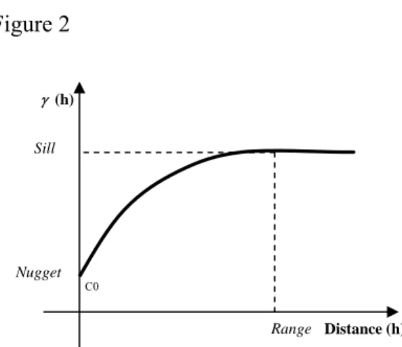
The SAC was checked separately for the four streams through the application of a semivariogram function. A variogram function (γ (h)) is a mathematical description that relates variance (or dissimilarity) of data points to a given attribute with the distance that separates them (Isaacs and Srivastava, 1989). Figure 2 shows the semivariogram function. The range is the distance where the model first flattens. Sample locations, SU in our case study, separated by distances closer than the range are spatially autocorrelated, whereas locations farther apart than the range, are not. Sill is the value of the semivariance as the lag (h) tends to infinity. The nugget effect can be attributed to measurement errors or spatial sources of variation at distances smaller than the sampling interval (or both). Ideally γ (0) = 0, but in practice, as h tends to 0, γ (h) tends to C0. Variation at microscales smaller than the sampling distances will appear as part of the nugget effect. For more detailed information about variogram functions see Cressie (1991), Wackernagel (2003) and Webster and Oliver (2007).
In order to describe the spatial component of the biological data we used the local Moran’s Index (Anselin, 1995), a measure of contagion that includes the effect of the spatial neighbourhood (Keitt et al., 2002; Segurado and Araújo, 2004). The local Moran’s Index has a value of SAC for each SU, rather than a single value (global Moran’s Index) for the entire data set. The spatial dependence of the land use variables was not evaluated, but by ensuring the spatial dependence of the biological variable, unbiased correlations between dependent and independent variables area guaranteed (Lennon, 2000).
2.4 Influence of land use in the riparian vegetation structure
The biological data set was subjected to constrained ordination procedures using CANOCO ver. 4.5 (ter Braak and Smilauer, 2002), to determine the influence of proximal and distal land use in explaining the patterns of the riparian vegetation structure. Detrended Correspondence Analysis (DCA) was used to choose the adequate type of model (linear or unimodal) for our data, through calculation of the gradient length (standard deviation units, SD, of species turnover). We obtained gradients lengths of 3.427 SD and 2.843 SD from the first two axes which led to the choice of the linear model (lengths are < 4 SD; Leps and Smilauer, 2003), Redundancy Analysis (RDA).
We used two approaches to verify the influence of the spatial component in our data. In the first one, we incorporated the spatial component in the biological data. RDA was performed: i) using solely land use variables ii) using the local Moran’s Index matrixas a covariable and iii) assessing the variation that results from the joint effect of the two sets of variables (spatial and land use components) In the second approach we removed the SAC, by using spatially independent SU. The distance between SU was defined by the values of the range obtained by an application of a semivariogram function to the riparian metrics. This is an alternative to avoid the SAC by “adopting a systematic scheme that constrains observations to be spaced far enough from each other” (Guisan and Theurillat, 2000). The method of assortment was chosen to maximize the data sample size, avoiding the duplication of any riparian unit. More precisely, the independent subsamples were obtained by using systematically one SU separated from the following one by the range value, so the first subsample includes the SU1, the second subsample begins in the SU2 and so forth.
In both approaches, the metrics data set was centred and standardized and the correlation matrix was used to make them comparable.
The total variance explained for each combination was obtained by the sum of all canonical eigenvalues. Variance inflation factors for the explanatory variables were examined and only the subset of the best predictors (by forward selection) that avoided the colinearity between variables was retained. The tests were performed for all vegetation classes.
Multiple linear regressions were implemented with STATISTICA software ver. 6.0 (StatSoft Inc., 2001) to model the relationship of land use variables and riparian vegetation structure. We used a forward selection and counted the number of times that each variable was significant (*P<0.05) in order to identify the best subset of land use variables, witch were the variables that contributed more to explaining the biological variation.
3. Results
3.1 Riparian structure
The study area encompasses 330 SU, which resulted in the delimitation of 3900 patches of riparian vegetation.
Table 2 summarizes the overall characteristics of the riparian structure using the landscape metrics. The tree cover class was the most abundant, and presented the largest patches when compared to the other riparian cover classes, though a higher variability of the patch size was also found. The highest number of tree cover patches was found in upstream SU of Sôr river, whereas lower numbers occurred close to urban areas and small farms or when the woodlands present consistently high riparian widths (at least more than 30 m). Metrics associated to the connectivity, namely the Mean Nearest-Neighbor Distance (MNN) and the Mean Proximity Index (MPI) allow the identification of a higher connectivity of tree cover class in comparison to the other cover classes. The higher values of Mean Fractal Dimension Index (MPFD) corresponded to complex shapes of the tree patches with meandering forms. Patch homogeneity, in this case, is often reduced by the existence of shadow patches and occurred in association with large riparian widths. For very small patches, MPFD values exceeded the maximum value referred in the bibliography and probably occurred due to computational limitations. However, this patch dimension is infrequent in the study area.
Concerning the herbaceous cover class, higher values of Mean Patch Size (MPS) occurred close to irrigation crops or associated to temporary sand deposits; also higher values of Mean Shape Index (MSI) were associated to the elongated shapes which were characteristic of this cover class.
The shrub cover class was widespread in the studied area, though presenting low values of Interspersion and Juxtaposition Index (IJI).
A cross-check with field observations revealed little differences in the abundance cover of the various classes in comparison to the photointerpretation, especially for the shrub and herbaceous cover due to local disturbances, such as sand extraction. However, for the major part of the study area the classification done by photo interpretation was considered trustworthy.
3.2 Spatial autocorrelation
The results obtained with global Moran’s Index (Table 3) indicated the presence of Spatial Autocorrelation (SAC) in the most part of the metrics. That means that riparian vegetation areas with reduced connectivity are next to other fragmented zones, and complex patches evenly distributed along riparian landscapes are next to others with the same spatial pattern. The MPI which assesses simultaneously the degree of fragmentation and the isolation of a given class has a spatial random pattern, except for the shrub cover class. The MNN also did not reveal a significant spatial cluster pattern. The various configurations of the spatial distance matrix showed differences in the spatial pattern for the studied metrics. For the tree cover class, the restriction of the neighbourhood, especially the use of contiguous SU, showed an increase of the SAC and of its significance. For the other cover classes, especially for the shrub cover class, this trend is less pronounced. This reveals some specific local spatial behaviors that are hidden in the global SAC assessment, and points to the lack of independence between SU.
As the result of the application of a semivariogram function to the riparian metrics we estimated the variability of the range between 2395m and 2963m for the four streams.
In order to ensure the independence of the spatial data we used the value of 3000 m between SU, which includes the range values of the various metrics within the studied area. A
subsampling with 28 SU was obtained and resulted in 9 combinations (for details see section 2.4).
3.3 Land use and spatial influence in the riparian vegetation structure
Table 4 shows the contribution of the land use variables to the total variance of the biological data obtained from Redundancy Analyses (RDA) using three data sets: solely land use variables, land use variables and spatial co-variables and land use and spatial variables. On the whole, the proximal land use data set (30m buffer) presented consistently higher values of the explained variance than the distal land use. Another consistent pattern that emerges on overall RDA analyses was the decrease of the explained variance with the removal of the spatial component.
The explained variation that results from the joint effect of the land use and spatial component ranged between 20.1% and 33.4%. This indicates that the riparian vegetation structure is more dependent on its spatial component than on the land use variables for both buffers. The tree cover revealed higher and more significant results (for the trace and for the eigenvalues)than the other vegetation classes across all RDA analysis.
Table 5 presents the results of the explained variance of the proximal and distal land use data set using the spatial independence sub-sampling. The explained variance of the land use variables increases with the spatial independence of the data, with average values ranging between 21.9% and 31.8%. The proximal land use presented also a higher influence on the biological variability than the distal land use buffer. The tree cover class was more influenced by the proximal land use than the other vegetation classes, whereas the distal land use had more influence in the herbaceous cover class than the shrub and tree cover classes; however a large variability between the different SU combinations was also detected.
3.4 Influence of land use variables in tree cover class
Tree cover class was used to evaluate the influence of land use, since it was better represented in the study area and displayed the highest percentage of variance on the overall RDA analysis than the other cover classes.
In general, the observed and the expected responses of landscape metrics to the increase of land use were concordant (Table 6). The agriculture followed by the agro-forestry were the variables with more influence in the tree cover class, and displayed a higher percentage of variance for the proximal than for the distal land-use buffer.
The number and the size of tree patches decreased with increasing land use pressure. The distance between riparian tree patches (given by the MNN) is higher and the connectivity (expressed by the MPI) is lower, showing an increasing fragmentation of the tree cover with the increasing land use pressure. However, opposite responses were found with the agro-forestry variable at both buffers. With increasing land use the Patch Size Coefficient of Variation (PSCV) points to a homogenization of the tree patches, suggesting a reduction of the intraspecific variability of the riparian structure. The two configuration metrics (MSI and Mean Fractal Dimension Index, MPFD) revealed a decrease in the complexity (less jagged shapes) and the reduction of the perimeter of the riparian tree shapes. In addition, as shown by the IJI, increasing land use pressures led to a high variability of the riparian patches.
Figure 3 represents the response of two metrics to the increase of the agricultural area for the 30 m buffer. The MPS presented lower values and low variability with the increase of the area occupied by agriculture. The same pattern was observed for the MSI, however with higher variability with increasing agricultural areas.
4. Discussion
4.1 Assessing riparian structure through landscape metrics
Numerous studies on ecology and management of riparian zones aspire to relate human disturbances in the surrounding landscapes with degradation of riparian vegetation (e.g. Baker et al., 2007, Malanson and Cramer, 1999). Field-based methods over large areas are very time consuming and often result in the lost of the overall perception of the landscape, thus frustrating the proposal of generalised management guidelines. Riparian structural attributes can be used as proxies of riparian width, longitudinal continuity and fragmentation (Johansen and Phinn, 2006), and therefore be considered potential indicators for riparian ecological quality. The present study uses a set of landscape metrics functionally skilled to assess quality of riparian zones and proposes a combined approach to characterize structural attributes at broad scale. Moreover, multiple-sided views of the riparian system were assessed using spatial metrics of patch configuration, isolation, inter-connectivity and distribution. In addition, the bi-dimensionality of riparian woods and the unique distribution within the landscape dictates a distinct analysis from those used for forest, croplands or natural vegetation patches. Besides the widely recognized need to combine metrics from the same functional category, such as the number and size of patches this study also revealed that a complementary approach on diverse functional group metrics contributes to a reliable appreciation of the riparian structure. For instance, spatial configuration metrics such as the Number of Patches and Mean Shape Index, jointly with connectivity metrics (e.g. Mean Nearest-Neighbour Distance, Mean Proximity Index) sheds light in the characterization of riparian structure. Particular spatial patterns of riparian vegetation were identified using landscape metrics. That is the case of wide well-preserved riparian woods which consistently displayed connected complex shapes, whereas the herbaceous vegetation, especially in
agricultural areas, has generally elongated simple shapes. These findings can help to identify highly degraded riparian corridors, invaded by the alien species giant reed, Arundo donax L., which generally present high connectivity patches, but simple stretched shapes. However, knowledge on the hydrogeomorphological background of streams is still indispensable, since narrow riparian woods naturally found in first order streams mimic the degraded riparian vegetation, with small linear patches with low inter-connectivity.
A limited ability of mapping and delineating riparian vegetation patches of the various considered strata was observed using the digital imagery with 0.5 x 0.5 m resolution, due to potential underestimation and misclassification of shrub and herbaceous strata. Most studies using remote sensing imagery considered the overall woody vegetation (e.g. Schuft et al.,1999; Apan et al., 2002), whereas for more detailed assessments, the characterization of the canopy and subcanopy surface topography is required and other remote sensing techniques are recommended, such as the LIDAR sensors, broad beam, full return with high sampling rates (Goetz, 2006).
4.2 Spatial autocorrelation assessment
Few riparian vegetation studies take into account the spatial autocorrelation of data (SAC), when relating variables that depend heavily, overall and locally, on their geographical location. For the characterization of riparian vegetation structure, most of metrics revealed a high global SAC, and also a high variability of local spatial dependence. Moreover, this is also dependent of the vegetation strata considered. Exceptionally, the connectivity metric Mean Patch Index showed a spatially random pattern for the tree layer, however, this could be explained by the selection of the connectivity threshold rather than by spatial independence of data distribution. The dependence patterns observed can be explained by historical factors
(Segurado et al., 2006; Dormann, 2007), biotic factors (Legendre, 1993), and may be the result of the spatial structure among environmental variables (Legendre and Fortin, 1989). This study also suggests a SAC evaluation procedure for the influence of the surrounding land use using two approaches; the incorporation of the spatial component in the riparian structure, and the use of spatial independent sampling units. The first procedure revealed a higher dependence of the spatial component, and a decrease of the explained variance of the land use variables with the removal of the spatial component. The later led to a significant increase, though a lost of biological information due to sub-sampling is unavoidable.
4.3 Influence of land use in the riparian vegetation structure
The spatial patterns of distribution of riparian vegetation vary with the identified gradient of land-use pressure. For low-impact land use cover, such as the Mediterranean agropastoral systems (mainly open cork/ holm oaklands and shrublands), tree patches increase in sinuosity, heterogeneity and inter-connectivity, whereas in the agricultural landscapes were characterized by a low number of small patches (low Number of Patches and Mean Patch Size values) with simple and homogenous shapes (low Mean Shape Index, Mean Patch Fractal Dimension and Patch Size Coefficient Variation values), less connected vegetation patches (high Mean Nearest Neighborhood Distance and low Mean Proximity Index values), and a non interspersed patch distribution (low Interspersion and Juxtaposition Index values). Timm et al. (2004), at the riparian areas of Cedar River, USA, considered highly fragmented riparian areas as having numerous and small patches, instead of reduced number of small patches. Both results fully represent the effects of the existing land use pressure, though fragmental patterns in our study area corresponded to a low riparian quality.
Similar fragmental patterns and connectivity loss related with increasing land use were found in other studies, such as the Ferreira et al. (2005), and Malanson and Cramer (1999); however, Apan et al. (2002) did not observed differences in spatial patch configurations (namely Mean Shape Index and Mean Patch Fractal Dimension values) possibly due to the coarse resolution of the mapping resources, which can alter the perceived capability of riparian attributes (Baker et al. 2007). Also, the results of the influence of two land use buffers agreed with conclusions of several studies (e.g. Bunn and Davies, 2000; Bott et al., 2006; von Schiller et al., 2008), and consubstantiate the suggestion of Aguiar and Ferreira (2005) for a major influence of the proximal land-use. In fact, an increment of around 22% of explained variability was achieved, when considering the influence of the 30 m buffer, instead of considering the all the river valley land use in the precursor study of Aguiar and Ferreira (2005). Even so, more than 60% of the biological variability remained without explanation. Natural disturbances, such has fire, and the hydrological torrential regime typical of Mediterranean rivers, as well as site-specific human disturbances such as the tree clearing, sand extraction, channel re-profiling can explain part of the riparian structure (McIntyre and Hobbs, 1999). Also, habitat variables especially from backsides (e.g. substrate, channel morphology) and the floristic composition, which were not considered in this study, could partially explain the riparian structure patterning. A natural/semi-natural vegetation cover and related riparian woody structure is required as a reference benchmark to further propose a predictive vegetation modelling based on land use changes.
5. Conclusion and implications for riparian management
This study suggests a consistent methodology to characterize riparian landscape structure and has demonstrated that metrics respond to different land use pressure, namely those related to the tree layer. Results also point to the need of considering the spatial component of the biological data, which is particularly relevant in riparian ecology, due to the linear nature of riparian vegetation. With the increased availability of GIS techniques this information can be stored and manipulated to produce tools for the management of the riparian zones. Landscape metrics can also consistently describe and quantify connectivity patterns for the riparian landscape, which are the surrogate of its ecological integrity. The fine scale resolution used for the detailed mapping of riparian structural attributes can be used to identify prioritizing reaches for conservation or rehabilitation. Finally, it is shown that land use in the area proximal to the riparian zones is determinant of the within-stand riparian structure therefore riparian protection areas should include the riparian zone and an adjacent buffer.
Acknowledgements
This study received backing from the project RIPIDURABLE “Gestion Durable de Ripisylves” (INTERREG III-C Sul - 3S0125I) and from the Forest Research Centre, CEF. We also want to acknowledge the Instituto Geográfico Português and the Autoridade Florestal Nacional, which has provided the airborne digital images through the FIGEE program.
6. References
Aguiar, F.C., Ferreira, M.T., Moreira, I., Albuquerque, A., 2000. Riparian types in Mediterranean basin. Aspects of Applied Biology 58, 221-232.
Aguiar, F.C., Ferreira, M.T., 2005. Human-disturbed landscapes: Effects on composition and integrity of riparian woody vegetation in the Tagus River basin, Portugal. Environmental Conservation 32 (1), 30–41.
Allan, J.D., 2004. Landscapes and Riverscapes: The influence of land use on stream ecosystems. Annual Review of Ecology and Systematics 35, 257-284.
Anselin, L., 1995. Local indicators of spatial association – LISA. Geographical Analysis 27, 93-115.
Anselin, L., 2002. Exploring Spatial Data with DynESDA2. CSISS and Spatial Analysis Laboratory University of Illinois, Urbana-Champaign.
Apan, A.A., Raine, S.R., Paterson, M.S., 2002. Mapping an analysis of changes in the riparian landscape structure of Lockyer Valley catchment Queensland, Australia. Landscape and Urban Planning 59, 43-57.
Baker, M.E., Weller, D.E., Jordan, T.E., 2007. Effects of stream map resolution on measures of riparian buffer distribution and nutrient potential. Landscape Ecology 27 (7), 973-992. Bott, T.L., Montgomery, D.S., Newbold, J.D., Arscott, D.B., Dow, C.L., Aufdenkampe, A.K., Jackson, J.K., Kaplan, L.A., 2006. Ecosystem metabolism in streams of the Catskill
Mountains (Delaware and Hudson River watersheds) and Lower Hudson Valley. Journal of the North American Benthological Society 25, 1018-1044.
ter Braak, C.J.F., Smilauer, P., 2002. CANOCO reference manual and CanoDraw for Windows user’s guide: software for canonical community ordination (version 4.5). Microcomputer Power, Ithaca, NY.
Bunn, S.E., Davies, P.M., 2000. Biological processes in running waters and their implications for the assessment of ecological integrity. Hydrobiologia, 442/443, 61-70.
Congalton, R.G., Birch, K., Jones, R., Schriever, J., 2002. Evaluating remotely sensed techniques for mapping riparian vegetation. Computers and Electronics in Agriculture 37, 113-126.
Corbacho, C., Sánchez, J.M., Costillo, E., 2003. Patterns of structural complexity and human disturbance of riparian vegetation in agricultural landscapes of Mediterranean area. Agriculture, Ecosystems and Environment 95, 495-507.
Cressie, N., 1991. Statistics for spatial data. John Wiley and Sons. New York.
Davis, P.A., Staid, M.I., Plescia, J.B., Johnson, J.R., 2002. Evaluation of airborne image data for mapping riparian vegetation within the Grand Canyon. Report of U.S.Geological Survey. Arizona.
Décamps, H., Fortune, M., Gazelle, F., Patou, G., 1988. Historical influence of man on the riparian dynamics of fluvial landscape. Landscape Ecology 1, 163-173.
Dixon, I., Douglas, M., Dowe, J., Burrows, D., 2006. Tropical rapid appraisal of riparian condition version 1. River management technical guidelines. No7 Land and Water Australia, Canberra, Australia.
Dormann, C.F., 2007. Effects of incorporating spatial autocorrelation into the analysis of species distribution data. Global Ecology and Biogeography 16, 129-138.
EU-WFD, 2000. European Commission Directive 2000/60/EC. European parliament of the council of 23 October 2000 establish a framework for Community action in the field of water policy. Official Journal of the European Communities L327.1-72.
Ferreira, M.T., Aguiar, F.C., Nogueira, C., 2005. Changes in riparian woods over space and time: Influence of environment and land use. Forest Ecology and Management 212 (1-3), 145-159.
Forman, R.T.T., 1997. Land Mosaics: The Ecology of Landscapes and Regions, Cambridge University Press, Cambridge.
Fortin, M-J., Dale, M.R.T., Hoef, J., 2002. Spatial analysis in Ecology. Encyclopedia of Environmetrics. JohnWiley , Sons, Ltd, Chichester. Vol 4, pp 2051-2058.
Goetz, S.J., 2006. Remote Sensing of Riparian Buffers: Past Progress and Future Prospects. Journal of the American Water Resources 2, 133-43.
González-del-Tánago, M., Garcia-Jalón, D., 2006. Attributes for assessing the environmental quality of riparian zones. Limnetica 25(1-2), 389-402.
Guisan, A., Theurillat, J.P., 2000. Assessing alpine plant vulnerability to climate change: a modelling perspective. Integrated Assessment 1, 307-320.
Isaacs, E.H., Srivastava, M., 1989. An Introduction to Applied Geostatistics. New York: Oxford University Press, pp 146.
Johansen, K., Phinn, S., 2006. Mapping Structural Parameters and Species Composition of Riparian Vegetation Using IKONOS and Landsat ETM+ Data in Australian Tropical Savannahs. Photogrammetric Engineering and Remote Sensing 72(1), 71-80.
Johansen, K., Coops, N.C., Gergel, S.E., Stange, Y., 2007. Application of high spatial resolution satellite imagery for riparian and forest ecosystem classification. Remote Sensing of Environment 110(1), 29-44.
Keitt, T.H., Bjornstad, O.N., Dixon, P.M., Citron-Pousty, S., 2002. Accounting for spatial pattern when modeling organism-environment interactions. Ecography 25, 616-625.
Legendre, P., Fortin, M., 1989. Spatial pattern and ecological analysis. Vegetatio 80, 107-138.
Legendre, P., 1993. Spatial autocorrelation: Trouble or new paradigm?. Ecology 74, 1659-1673.
Lennon, J.J., 2000. Red-shifts and red herrings in geographical ecology. Ecography 23, 101-113.
Leps, J., Smilauer, P., 2003. Multivariate analysis of Ecological Data using CANOCO. Cambridge University Press, Cambridge, UK.
Looy, K.V., Meire, P., Wasson, J.G., 2008. Including riparian vegetation in the definition of morphologic reference conditions for large rivers: a case study for europe’s western plains. Environmental Management 41, 625-639.
Main, C.L., Robinson, D.K., McElroy, J.S., Mueller, T.C., 2004. A guide to predicting spatial distribution of weed emergence using geographic information systems (GIS). Applied Turfgrass Science. online. doi:10.1094/ATS-2004-1025-01-DG.
Malanson, G.P., Cramer, B.E., 1999. Landscape heterogeneity, connectivity and critical landscapes for conservation. Diversity and Distributions 5, 27-39.
McGarigal, K., Marks, B.J., 1994. FRAGSTATS “Spatial Pattern Analysis Program for Quantifying Landscape Structure”. Forest Science Department, Oregon State University, Corvallis.
McIntyre, S., Hobbs, R.A., 1999. A framework for conceptualizing human effects on landscapes and its relevance to management and research models. Conservation Biology 13(6), 1282-1292.
Miller, J., Franklin, J., Aspinall, R., 2007. Incorporating spatial dependence in predictive vegetation models. Ecological Modelling 202, 225-242.
Moran, P.A.P., 1950. Notes on continuous stochastic phenomena. Biometrika 37, 17-23.
Muller, E., 1997. Mapping riparian vegetation along rivers: old concepts and new methods. Aquatic Botany 58, 411-437.
Naiman, R.J., Décamps, H., 1997. The ecology of interfaces: riparian zones. Annual Review of Ecology and Systemstics 28, 621-658.
Rex, K.D., Malanson, G.P., 1990. The fractal shape of riparian patches. Landscape Ecology 4, 249-258.
von Schiller, D., Martí, E., Riera, J.L., Ribot, M., Marks, J.C., Sabater, F., 2008. Influence of land use on stream ecosystem function in a Mediterranean catchment. Freshwater Biology 53, 2600-2612.
Schuft, M.J., Moser, T.J., Wigington, P.J., Stevens, D.L., McAllister, L.S., Chapman, S.S., Ernst, T.L., 1999. Development of landscape metrics for characterizing riparian-stream networks. Photogrammetric Engineering and Remote Sensing 65(10), 1157-1167.
Segurado, P., Araújo, M.B., 2004. An evaluation of methods for modelling species distributions. Journal of Biogeography 31, 1555-1568.
Segurado, P., Araújo, M.B., Kunin, E., 2006. Consequences of spatial autocorrelation for niche-based models. Journal of Applied Ecology 43, 433-444.
StatSoft, Inc., 2001. STATISTICA (data analysis software system), version 6. www.statsoft.com.
Stromberg, J.C., 1993. Instream flow models for mixed deciduous riparian vegetation within a semi-arid region. Regulated Rivers: Research and Management 8, 225-235.
Timm, R.K., Small, J.W., Leschine, T.M., Lucchetti, G., 2004. A screening procedure for prioritizing riparian management. Environmental Management 33(1), 151-161.
Tobler, W., 1979. “Cellular geography”. In Miller, J. Franklin J., Aspinall, R., 2007. Incorporating spatial dependence in predictive vegetation models. Ecological Modeling 202, 225-242.
Turner, M.G., 1989. Landscape ecology: the effect of pattern on process. Annual Review of Ecology and Systematics 20, 171-197.
Wackernagel, H., 2003. Multivariate Geostatistics: an Introduction with applications. (3rd ed.). Berlin. Springer.
Ward, T.A., Tate, K.W., Atwill, E.R., 2003. Visual assessment of riparian health. Rangeland Monotoring Series, Publication 8089. University of California.
Webster, R., Oliver, M.A., 2007. Geostatistics for Environmental Scientists. John Wiley and Sons. (2nd ed.).
Yang, X., 2007. Integrated of remote sensing and geographic information systems in riparian vegetation delineation and mapping. International Journal of Remote Sensing 28(2), 353-370.
Table 1. Metrics, acronyms, units, range, description (formulae and detailed calculation from McGarigal and Marks, 1994) and implications in the characterization of riparian vegetation structure.
Metrics Acronym Units and
range Description Implications
Number of
Patches NP None [1, ∞]
Mean Patch Size MPS Square
meters ]0, ∞]
Basic statistics of the spatial configuration
Simple indicators of the riparian fragmentation Patch Size Coefficient of Variation PSCV Percentage [0, ∞]
Variability in the size of the patches Heterogeneity of the riparian structure Mean Shape Index MSI None [1, ∞] Complexity of shapes. Approaches 1 for shapes with simple perimeters. Mean Fractal Dimension Index MPFD None [1,2]
Fractal dimension: ratio of perimeter per unit area. Increases as the patches become more irregular
Spatial configuration of the riparian woods in terms of complexity of vegetation patches Mean Nearest-Neighbor Distance MNN Meters ]0, ∞] Minimum distance between patches of the same class, based on the shortest distance between their edges Isolation of vegetation patches. Inter-connectivity of riparian structure Mean Proximity Index Connectivity MPI None [0, ∞]
Increases as the patches of the corresponding patch type become less isolated and less fragmented.
Degree of isolation and fragmentation to a given class Interspersion and Juxtaposition Index IJI Percentage ]0,100] Proximity of patches in each class. High values correspond to
proportionate distribution of patch type adjacencies
Distribution of vegetation patches
Table 2. Minimum and maximum values, average ± SD (in parentheses) for the tree, shrub and herbaceous cover classes per Sampling Unit. Metric acronyms are given in Table 1. Cover classes: Tcov- tree, Scov – shrub, Hcov-herbaceous.
Metric Tcov Scov Hcov
NP 1.00 – 14.00 (3.43 ± 2.29) 1.00 - 11.00 (2.23 ± 1.62) 1.00 - 8.00 (1.92 ± 1.12) MPS 21.67 - 11268.02 (1000.57 ±1387.17) 5.41 - 4770.42 (413.94 ± 626.97) 6.73- 2183.67 (420.70 ± 501.30) PSCV 6.60 - 211.81 (84.29 ±41.10) 2.67 - 151.54 (63.20 ± 34.03) 9.01 - 128.58 (57.57 ± 30.49) MSI 1.03 - 5.47 (2.00 ± 0.76) 1.08 - 4.15 (1.79 ± 0.57) 1.16 -5.70 (2.12 ± 0.93) MPFD 1.47 - 2.13 (1.69 ± 0.11) 1.46 - 2.67 (1.73 ±0.17) 1.45- 2.69 (1.78 ± 0.17) MNN 0.37 - 171.70 (15.10 ± 23.94) 0.80 - 210.70 (34.49 ± 45.13) 1.80 - 134.50 (28.35 ± 29.29) MPI 2.43 - 4584.94 (379.34 ± 651.59) 1.12 - 539.37 (81.96 ± 126.11) 2.26 - 114.37 (25.35 ± 28.15) IJI 0.00 - 22.66 (10.00 ±5.37) 1.27 - 24.99 (11.63 ± 4.89) 0.00 - 19.97 (8.91± 5.71)
Table 3 .Moran’s I and z-scores for the riparian metrics, using different configurations of the spatial proximity matrix. Significant cluster patterns are indicated in bold, random patterns are indicated as R (**P<0.01). Metric acronyms are given in Table1. Cover classes: Tcov- tree, Scov – shrub, Hcov-herbaceous.
Configuration criteria Metric
Inverse distance Threshold distance (1000m) First continuity order Tcov Scov Hcov Tcov Scov Hcov Tcov Scov Hcov NP 0.16 4.42 0.21 4.41 0.1R 1.77 0.23 4.35 0.31 4.17 0.22 7.69 0.36 7.44 0.17 2.90 0.43 6.22 MPS 0.18 5.27 0.09R 1.78 0.38 6.75 0.26 5.02 0.10 4.45 0.22 7.69 0.39 8.24 0.20 3.38 0.43 6.22 PSCV 0.17 4.75 0.12 2.38 0.01R 0.32 0.24 4.55 0.02R 0.90 -0.01R -0.23 0.23 4.70 0.13 2.10 0.11R 1.70 MSI 0.20 5.73 -0.06R -1.10 0.32 5.62 0.30 5.69 0.06 2.51 0.31 11.07 0.35 7.31 0.14 2.38 0.51 7.38 MPFD 0.17 4.84 0.28 5.52 0.45 8.00 0.25 4.71 0.19 7.68 0.26 9.27 0.26 5.07 0.37 6.09 0.49 7.11 MNN 0.01R 0.30 0R 0.18 0.11 2.07 0.01 0.21 0.02R 1.00 -0.03R -0.99 0.01 0.21 0.09R 1.55 0.01 0.25 MPI 0.04 1.26 0.14 3.07 0R 0.11 0.05 1.06 0.01R 0.48 0.01R 0.77 0.03 0.82 0.11 2.11 0.00R 0.16 IJI 0.25 6.93 0.13 2.59 0.16 2.89 0.37 6.84 0.04 1.97 0.21 7.71 0.48 10.03 0.19 3.12 0.42 6.16
Table 4. Contribution to total variance (%) of explanatory variables using RDA with solely land use variables, land use variables and spatial co-variables and land use and spatial variables, per vegetation class (n=330) with the 30 and3 200 m buffers. Cover classes: Tcov- tree, Scov – shrub, Hcov-herbaceous.
Land use variables
Land use variables + spatial covariables
Land use + spatial variables Cover class 30 200 30 200 30 200 Tcov 13.1 3.6 7.4 1.8 33.4 28.2 Scov 4.5 2.3 4.3 0.6 20.9 20.1 Hcov 4.7 2.9 2.2 1.3 23.0 22.1 Tcov+Scov+Hcov 7.5 3.0 4.5 1.6 32.2 29.4
Table 5. Minimum and maximum values, average ± SD (in parentheses) of the contribution to total variance (%) of land use variables per cover class, using non-autocorrelated SU (9 combinations, n=28) in 30 and 200 m buffers. Cover classes: Tcov- tree, Scov – shrub, Hcov-herbaceous. Buffer Cover class 30 m 200 m Tcov 27.4 - 37.8 (31.8 ± 3.0) 13.6 – 29.6 (18.2 ± 5.2) Scov 16.1 – 28.1 (21.9 ± 4.1) 12.3 – 25.2 (19.6 ± 4.1) Hcov 21.6 – 36 (27.4 ± 5.1) 10.3 – 31.1 (23.1 ± 6.3) Tcov+Scov+Hcov 23.0 – 30.6 (27.1 ±2.6) 14.6 – 24.3 (19.9 ± 3.2)
Table 6. Expected and observed responses to land use increase (Ç- positive relation, È - negative relation) and number of significant multiple regression analysis (*P<0.05) in the 30 and 200 m buffers. Metric acronyms are given in Table 1.
Observed response
Agriculture Agro-forestry Forestry Impervious Roads
Metric Expected response 30 200 30 200 30 200 30 200 30 200 NP È È 5 È 1 Ç 1 È 1 MPS È È 7 È 3 PSCV È È 4 È 1 È 1 È1 È 1 Ç 1 MSI È È 6 È 1 È 2 MPFD È È 3 È 1 È 1 È 1 È 1 È 1 MNN Ç Ç 1 Ç 2 È 1 Ç1 Ç 1 Ç 1 MPI È È 2 È 1 Ç 1 È 1 È 1 Ç 1 IJI È È 7 È 1 È 2 Ç1 È 1 È 2 Ç 1 Significant regression analysis (nº.) 34 7 13 3 3 2 2 3 3 3
Figure 1. Iberian Peninsula, showing the Portuguese part of the Tagus basin and the location of the four river basins
Figure 2. Semivariogram function (adapted from Main et al., 2004)
Figure 3. Median, 25 and 75 quartile for the Mean Patch Size (MPS) and Mean Shape Index (MSI) of the tree cover class with the increase of the agricultural areas in the 30 m buffer (n=28 SU, 9 combinations ).
Figure 2 Range γ (h) Distance (h) Nugget Sill C0
Figure 3 0 400 800 1200 1600 MPS_Tree (m 2 ) 0,0 0,5 1,0 1,5 2,0 2,5 MSI_Tree 25 50 75 100 Agriculture (%)