d-array beamforming during
ship's
noeuvring
P.Felisberto S.M. Jesus
Indexing terms: Hydrophone uvvays, Array shape distoriion
Abstract: Towed hydrophone arrays are
commonly used for determining the spatial characteristics of the underwater acoustic field. The assumption that the hydrophones lie in a straight and horizontal line is often made when beamforming the hydrophone outputs. However. due to tow vessel motion, ocean swells and currents the array adopts a nonlinear shape and the beamformer output is degraded. To estimate the positions of the hydrophones an array was instrumented with a set of positioning sensors: compasses, tiltmeters, accelerometers and pressure
gauges. The authors present the array
deformations recorded at sea when the tow vessel is turning and along straight-line tracks. The influence of the observed deformations on the performance of the conventional beamformer output is discussed and illustrated with simulated and real acoustic data.
1 Introduction
Towed arrays are widely used in underwater acoustics for estimating the horizontal directionality of the acoustic field. Fast plane-wave beamforming algo- rithms require the assumption that the array is straight and horizontal. The underlying justification is that the use of an equispaced and straight-line array allows to important algorithmic simplifications leading to a dra- matic increase of computing efficiency. Unfortunately, this assumption is not always fully verified in practice. In fact due to tow ship speed and course fluctuations, underwater currents, swell and other effects the array shape is often far from linear. It is true that the devia- tions from the linear shape are also dependent on the array construction parameters like length, thickness, number of mechanical sections and him liaisons. When the array deviates from the assumed linear shape, the beamformer output performance is degraded with bear- ing estimation errors, loss of beam power and increased sidelobe levels. However, this problem can be avoided if the hydrophone positions can be estimated and the respective corrections introduced in the beamformer.
0 IEE, 1996
IEE Proceedings online no. 19960492
Paper first received 29th September 1995 and in revised form 21st March
1996
The authors are with UCEH ~ University of Algarve. Campus de
Gdmbelas, PT-8000 Faro, Portugal
Generally, two types of method were used to estimate the acoustic sensor positions on a perturbed array. In the first type, the array is instrumented with position- ing sensors such as compasses, tiltmeters, pressure gauges and then some interpolation scheme is used to determine the hydrophone positions [l]. Methods of the second kind are known as data driven since they estimate the hydrophone positions from the acoustic data itself. These methods do not need any additional positioning sensors mounted on the array, but array shape estimation is, in these cases, highly time consum- ing and sometimes sources at known far-field locations are needed [2-71.
In this paper we estimate hydrophone array deforma- tions based on the information recorded at sea with a 156m-length array instrumented with several position- ing modules. The nonacoustic data and the interpola- tion scheme used to estimate the hydrophone positions is presented. Beamformer outputs are compared in dif- ferent tow ship's manoeuvring situations to analyse the influence of the array deviations from linearity. This work also addresses the problem of estimating the acoustic field directionality in the full 0-360" range.
.Isource
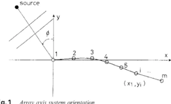
Fig. 1 Arruy axis .ry.rfem orientation
2
Beamforming is a well known technique to observe the directionality of the acoustic field sampled by an hydrophone array. To observe signals from a given direction the beamformer coherently adds the hydro- phone outputs by adjusting their relative delays for that direction. Frequently, beamforming is performed in the frequency domain, in which case the relative delays are replaced by the equivalent phases. Consider a plane wave impinging at bearing
9,
on a towed array with M hydrophones uniformly spaced at d metres as shown in Fig. 1. Our interest concentrates on the azi- muthal bearing, thus only the deformations in the xy-plane are considered. In the frequency domain, theBeamforming of deformed towed array
IEE Proc -Radar, Sonar Navig., Vol. 143, No. 3, June 1996 210
beamforming operation for a given I frequency bin can be written as [3]
G/,$ = (1)
where X , , denotes the o1 frequency component of the observation at hydrophone I, c is the sound speed, M is the number of sensors and (xnf, y,) is mth hydrophone position. Source bearing is estimated by finding the value of (I that maximises eqn. 1. Generally, an imple- mentation of eqn. 1 is computationally intensive but it can be enhanced if the assumption that
x,
= md is made (i.e. assuming that the disturbance along the x- axis can be neglected). Defining the normalised spatial frequency (or wavenumber) k asIt!-1
W1
X L , ~ exp - j - { x m sin
4
- ym cos q5}m = O
Thus, rewriting G as function of wavenumber k and using the approximation x,, = und
( 3 )
(4) These expressions can be implemented more efficiently than eqn. 1 if some symmetries and similarities are explored. From this point of view the most favourable case occurs when the array is straight and horizontal (all
Y~
= 0) in which case an F F T algorithm can be applied. To have an idea of the quality of the approxi- mation, a comparative study between the outputs from the approximated method (eqns. 3 and 4) and the gen- eralised method (eqn. 1) has been made. This study showed that the approximated beampattern could not be distinguished from the true beampattern for sources at or near broadside and showed a maximum error of 5dB for sources at or near endfire. That behaviour is approximately constant for any frequency below the maximum array working frequency.A well known drawback of the straight-line array assumption is the left- right ambiguity. This ambiguity arises because the relative delays between sensors for a chosen source bearing are the same regardless of the source’s left--right position. When the array is deformed this no longer happens and therefore the ambiguity problem can be solved. Analysing GP and
GN, observe that the joining maximum occurs in GP if the source is in the right side of the array. The opposite happens for GN that peaks for a source in the left side of the array.
3 Estimating array deformation
A sketch of the array used in the experiment is depicted in Fig. 2. The array has 40 uniformly spaced hydro- I b 6 Proc -Radar, Sonut Nuvig Vol 143 No 3 June 1996
phones at 4m, placed in three acoustic mechanical sec- tions and a tail element. To determine the hydrophone positions the array was instrumented with the following set of positioning sensors:
- six tiltmeters (TI to T6)
six compasses (Cl to C6) six accelerometers (A 1 to A6) two pressure gauges
head tail
32rn 32m 32m 32m 32m 32m 5m
i
-4
C-T-Ai c-T-&/ C-T-A; p-c-T-Abj acoustic section 1 acoustic section 2 acoustic section 3Fig. 2
C = compasses, T Towed array = tiltmeters, A configurution and = accelerometers, positioning modules P = pressure gauges
The pressure gauges were installed one in the array head and the other in the array tail. The compass C1, the tiltmeter T I and the accelerometer A1 that form the first positioning module were installed nearby the hydrophone closest to the ship (no. 1). That hydro- phone was chosen as the origin of the Cartesian posi- tioning system. In this system, it is assumed that the x- axis and the first compass direction are colinear. The absolute angles measured by the others compasses (C2 to C6) are transformed in relative angles to the x-axis by subtracting the values from compass C1. The posi- tioning modules (each composed of one compass, one tiltmeter and one accelerometer) were placed at 32m intervals. To estirnate the hydrophone’s positions in between two adjacent modules a linear interpolation scheme with a 0.5, griding was used. Consider the vector (c1, c2, ..., clV) as the interpolated compass values and the vector ( t l , t2, ..., tN) as the interpolated tiltme- ter values; N is the number of interpolation samples.
To estimate the three dimensional coordinates xi, yi, zi;
i = 1, ..., N , the following expressions were used
x; = 5;-1
+
b cos4%
cos A; yz = yi-1+
S
cos q$ sin A;zi = z,-1
+
6sin q5i( 5 )
where X I = 0, y1 = 0, z1 = 0, 6 = 0.5m is the interpola- tion interval and the angles were computed using
The hydrophone positions are a subset of the com- puted values for i = 1, 9, 17, 25, .... This is a very sim- ple procedure that can be easily implemented in a real- time system with inexpensive hardware. Note that the z-co-ordinate is estimated here, but for our purposes only the x- and y-co-ordinates were used when comput- ing the beamformer output described in Section 2. Also, if the absolute depth is needed then these algo- rithms can be combined with the measurements obtained from the array head and tail pressure gauges. Initially the installation of accelerometers was decided based on the observation that accelerations might be necessary to correct tiltmeter outputs since tiltmeters act like pendulums and are therefore very sensitive to accelerations. During the cruise a strong bias was observed on the accelerometer data and no correction seemed to be necessary on the tiltmeter outputs. In the sequel we concentrate on the compass-tiltmeter data.
4 At-sea data acquisition and processing
-81
4.
I
Tow-vessel navigation data
The sea trial took place in the Strait of Sicily in the Pantelleria area. Figs. 3-5 give a general view of the tow vessel navigation data during day 04 of March 1994. The ship made two 180" port turns. At these moments we expect significant disturbances in the array shape. Another navigation parameter that is important in the array deformation is the ship's speed. As can be seen the ship's speed fluctuations are rela- tively small during straight-line tracks and showed some variability only during the turns.
37 04 00" 37 03 30"/ OO. 37 03 $ 3 7 0 2 3 37 02 5 37 01
-
37 01 37 00 37 00 - longitude Fig.3 track inShp nubigation data during yea trial day 04 March 1994 h p
0
0 9 2 0 09:40 1O:OO 10:20 10:40 11.00 11 20 time, h:min
Ship nuvigation &tu during sea trial day 04 March 1994: sliip
50[
Y
Fig.4 c o u m in I O -- I OL 09 20 09 40 10 00 1020 1040 11 00 11 20 time, h rninFig.5 Shi navigation data during sea trial day 04 March 1994 ship ground ~ p e e j m
4.2
Array positioning data
The positioning sensor data was acquired with a sam- pling rate of one sample per second. Output examples of positioning sensor data for the time interval 09:07 to 11:38 are presented in Figs. 6-8. Fig. 6 shows the out- put data for one compass. The compasses diagrams are delayed replicas of the ship's course plot (Fig. 4). Data from one of the tiltmeters are shown in Fig. 7. These 212
data needed to be filtered to eliminate the high fre- quency components that are possibly due to flow noise. Also, from this plot the moments where the tow vessel turns are perceivable. Fig. 8 presents data from the pressure gauge located in array head, after conversion to depth. From this curve one can easily perceive when ship is turning. The output data from the other pres- sure gauge (located in the array tail) has a similar evo- lution with a constant bias (about lorn), even during turns. 3501 I ,OOt
L
2002501 i
I 09:07 09:57 time 10:47 11 38Fig. 6 Positioning data: compass
6 4 2
-4t
-6 6 5 , 601 55; I 20- 09 16 09'33 09'50 10 06 10'23 10'40 10 56 1113 11'30' time,h minFig.8 Positioning data pressure gauge
4.3
Estimated array deformation from
recorded positioning data
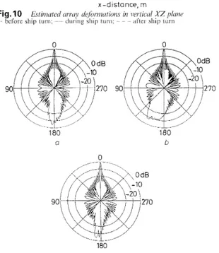
The array deformation was estimated using the proce- dure proposed in Section 3. Figs 9 and 10 illustrate a set of representative array shapes recorded before the turn (dotted line), during the turn (dashdot line) and after the turn (dashed line).
-
c c" -20 U - ! L -301 0 20 40 60 80 100 120 140 160Estimated array deformations in horizontal XYplane
x-distance, rn Fig. 9
before ship turn; - - during ship turn; - - - after ship turn
N
0 20 40 60 80 100 120 140 150
x-distance, m
Fig. 10 Estiniated w u y i:le$irnzutiulzs in vertical X Z plane '. before ship turn; ~ ~ during ship turn; ~ ~ ~ n f k r ship turn
(I U 0 /-I- - 180 b B 90 70 180 C Fig. 1 1
tions according to Figs. 9 and I O
(a) Bcfore ship turn (b) Duriiig ship t u n (c) After ship turn
Becm patterns j b r U bIYJUdSide s o u r c ~ will? real c i r r q ck$)rrw-
The spatial filtering characteristics of an array are sometimes illustrated by the beam power pattern. In Fig. 11 the normalised bcam power patterns are plotted according to the array deformations of Figs. 9 and 10 for the maximum working frequency o f the array
(187.5Hz) without steering. Depending on the level of array deformation the beam power pattern for the por- tion of the plane complementary to the source has a lower main lobe but a larger beam width, something like a shade. This is the starting point to solve the right-left ambiguity problem. From these Figures a dif- ference of up to 8dB between the main lobe and the shade can be noted. It can be shown that for the array considered and its observed deformations this differ- ence generally increases with array deformation, and the greater values are observed when the source is broadside to the array and its frequency is close to the array maximum working frequency. Since plots in Fig. 11 represent the theoretical beam power patterns for the deformations considered, it is expected that in real world, owing to sensor errors, related array shape estimation crrors and other errors, the difference between the main lobe and the shade is somehow smaller than the theoretical.
4.4
Processing acoustic data
Real acoustic data has been processed with the beam- forming expressions (eqns. 3 and 4), which are approx- imations o f eqn. 1 . As an example of the application to field data, a few observations recorded at one minute intervals during the second ship turn between 11:OS and l1:OX a.m. are presented in Figs. 12-23. The sam- pling frequency was 750Hz and the block size used for IEE Proc.-Radar, Sonar Nuvi,q. Vol. 143, hro. 3. June 1996
F F T computation was equal to 1024 samples. No aver- aging was done and the number of beams was equal to 128. During that experiment the ship was simultane- ously towing an array and an acoustic source emitting tones at 100, 120 and 12SHz. The acoustic field is essentially composed of the towed source signal at bearing 90" and a strong nearby merchant ship echo, covering the frequency range from 60 to 180Hz, close to broadside. There are a number of other minor noise sources, possibly owing to distant ships close to end- fire. 40 20 E O >; -20 -40 0 20 40 60 80 100 120 140 160 x, m
Fig. 12 Field lowed-array data at 11:05 am: sy-platie array deformation
20 LO 60 80 100 120 1LO 150 '180
frequency, Hz Fig. 16
siruight-line usray Field towetl-orrq
(/(itti 111 11:06 m i Ikwinjoriiiei. ourput .for
180
.-
20 -6 -8 -1 c -1 2 -1 4 -1 F -1 E -2c I I I I I I I I E 2; O. -20 I-
In Figs. 12-14, with an almost straight-line array, the strong ship echo at IO" can be clearly seen together with the three towed source tones. The 360" plot Fig. 14 shows that the left-right ambiguity cannot be resolved. Figs. 15-23, with a progressive array defor- mation. show that the strong ship echo is smeared on Figs. 16. 19 and 22 (that assumes a straight-line array) and the towed source tones cannot be distinguished from background noise. Simultaneously, the 360" plots show an increasing difference on the acoustic field received from the left and right sides of the array. A close analysis of this difference confirms that the strong ship echo is effectively located starboard at 10, 0, -10 and -45" from Figs. 14, 17, 20, 23, respectively.
40 20 E h 0 -20 -4 0 0 20 40 60 80 100 120 140 160 -LU" d 0
The sequcnce of observed array deformations are illustrated in Figs. 12, 15, 18 and 21. One can say that the array deformation is progressively increasing in the xy-plane up to 38m deviation at the array tail relative to the first hydrophone. Along this sequence, Figs. 13, 16, 19 and 22 show the beamformer output assuming a straight-line array. Figs. 14, 17, 20 and 23 present the beamformer output using eqns. 3 and 4 with the esti- mated array deformations shown in Figs. 13, 15. 18 and 21, respectively. In the 360" plots, frequency increases linearly from zero in the centre to 187.5Hz (the maximum working frequency) in the border. 214 -2 -4 -5 -8 0 A3 -10 0 m -1 2 -1 & -1 6 -1 a ^ ^ 5 Conclusions
This paper has shown a number of nonacoustic meas- urements aimed at estimating towed-array deforma- tions at sea. According to these observations it can be concluded that a towed array is never straight nor hor- izontal. As expected, this deviation from linearity is higher when the ship turns. In this case the beamformer output is highly reduced, inducing bearing estimation errors, loss of beam power and increased sidelobe lev- els. This paper presents a simple and fast method to estimate the array deformation based on nonacoustic positioning data recorded in real time and to include the deformation into the beamformer. It is shown that, depending on the deformation of the array, the left- right ambiguity can be resolved. The proposed models IEE froc.-Raclur, Sonar Ncivig., Vol. 143, No. 3, June 1996
to estimate the array shape and the acoustic field direc- tionality were successfully applied to real data where right and left sources could be unambiguously located on a 0-360” ring.
6 Acknowledgments
The authors acknowledge A . Kristensen and A. Caiti, scientists in charge, the master and crew of the RIV
Alliunce and the SACLANT Centre Engineering Department for their outstanding respective contribu- tions in the leadership, sea-going operation and cquip- ment preparation before and during the sea trial. The support of E. Dias and E. Coelho from the Hydro- graphic Institute, Lisbon, on the acquisition of the non- acoustic data is also appreciated. This work was supported by the Marine Science and Technology
(MAST 11) programme of EC under contract MAS2- CT920022.
7 References
1 HOWARD, B.E., and SYCK. J.M.: ‘Calculation of the shape of towed underwater acoustic array’, IEEE J . Oceaiz Eng., 1992, 17,
pp. 193-203
BUCKER, H.P.: ‘Beamforming a towed line array of unknown shape’, J. Acoust. Soc. Anter., 1978, 63. pp. 1451-1454
WAHL, D.E.: ‘Towed array shape estimation using frequency wavenumber da1.a’. IEEE J. Oceun. Eizg.. 1993. 18; pp. 532-590 BOUVET, M.: ‘Beamforming of a distorted line array in the pres- ence of uncertainties on the sensor positions’, J . Acoust. Soc. Amer., 1987, 81, pp, 1833-1840
5 FERGUSON, E.G.: ‘Sharpness applied to the adaptive bcam- forming of acoustic data’, J. Atoust. Soc. Amer., 1990, 88. pp. 2695-2701
6 QUINN, B.G., BARRETT, R.F., KOOTSOOKOS, P.J., and SEARLE, S.J.: .The estimation of the shape of an array using a hidden Markov model’. IEEE J . Ocean. Eng., 1993, 18, pp. 557- 564
7 FERGUSON, B.G.: ‘Remedying the effects of array shape distor- tion on the spatial filtering of acoustic data from a line array of hydrophones’, ZEEE J. Ocem. Eng., 1993. 18, pp. 565-571 GAO, S.-W., and GRIFFITHS, J.W.R.: ‘Experimental perform- ance of high-resolution array processing algorithms in a towed sonar array enviroiiment’, .I. Acoust. Soc. Amer., 1994, 95, pp. 2068-2080
2 3 4
8