Procedural aging techniques of synthetic cities and 3D scenarios

(1)

Procedural Aging Techniques of Synthetic Cities

and 3D Scenarios

Samuel Ferreira Dias

Dissertação para obtenção do Grau de Mestre em

Engenharia Informática

(2º ciclo de estudos)

Orientador: Prof. Doutor Abel Gomes

(2)

(3)

(4)

(5)

Acknowledgements

This was without doubt the biggest and the most challenging project I have already done in my entire live. This project made me overcome so many barriers and so many challenges, but none of this would be possible if I had not by my side the help of some people, so this text is for them.

Gratitude is the feeling that I’ll have forever to those who have helped me on this journey. This is the feeling that best represents what I feel for each of you and all that you contributed to my success.

First of all, I want to thank my supervisor, Prof. Abel Gomes, for all the support he gave me, because without it this journey would not have the foundation to reach the end. Mother and father, I want to thank you from my heart for all the support you gave me and for all the hard work you have done for me. You are without a doubt the most important people in my life because you always supported my decisions, gave me all the support I needed and especially were always by my side, so I never missed anything! I would not know what I would do without you. I will be forever grateful for all the spirit of sacrifice and love you had for me! I will never forget you!

Inês, I want to thank you for for all the support and help that you gave me. With small rocks we build a house, not being need something very big but yes something of quality! Thank you for helping me whenever I needed and for never having refused my needs. Thanks a lot for your help!

Maria Miguel, my love, what can I say of my source of happiness? Would last words, paragraphs, leaves to describe how important your help was for me during my journey. I want to thank you for all your support and help you have given me. You were without a doubt the great cause of my smile, Thank you also for your loving look! Thanks for our games and for making me happy. Thank you for showing me more than a way of doing and seeing things, because there is not always a single way of doing things and you often helped me to get over it and to open new horizons! Thank you for loving me unconditionally! Thank you for being the person that you are for me and for being the strong woman you are. Thanks for always being there for me always! Thank you for always being there always with a smile and a caring hug! Thank you! You let me inspire and you make go beyond! I love you! An eternal thanks!

My family and my friends, I want to thank all of them who helped me and accompanied me on this my journey. That sometimes heard me, and discussed my ideas and always lead me in the right way. A big thanks to all of you.

(6)

(7)

Resumo

Hoje em dia vivemos num mundo cada vez mais computorizado e exigente. Um mundo onde cada vez mais está presente a necessidade de a industria dos jogos de vídeo e dos filmes arranjar maneiras de criar ambientes gráficos mais realistas, mais rapidamente e já com um nível de variedade grande. Para colmatar esta necessidade surgiu então as técnicas de geração procedural. Estas técnicas aliaram-se á industria de computação gráfica para criar texturas naturais, simular efeitos especiais e gerar modelos naturais complexos, incluindo maioritariamente vegetação. Dentro destas primeiras técnicas podemos encontrar as fractais, L-system e Perlin Noise, entre outros. Posteriormente, com a necessidades de criar cada vez mais ambientes mais complexos, surgiu a solução de adaptar estes algoritmos já conhecidos para algo mais complexo, como a geração de uma estrutura rodoviária, ou como a geração de edifícios podendo assim praticamente gerar um mundo inteiro somente com a geração procedural e um conjunto de regras. Apesar de esta evolução ser cada vez mais sentida, notou-se um crescente interesse num tema em partcular, sendo essa, o envelhecimento procedural dos edifícios nestes mundos gráficos. Vários autores até então tinham-se proposto a criar novos e cada vez melhores algoritmos de envelhecimento procedural dos edifícios. Estes autores ao abordar este tema, tendem em seguir um caminho muito singular e especifico, criando um algoritmo capaz de reproduzir um unico fenomeno de envelhecimento.

Assim, identificada esta lacuna na literatura, decidiu-se agarrar esta oportunidade e apresentar e desenvolver um algoritmo de envelhecimento procedural aplicado aos ed-ifícios que é capaz de reproduzir diferentes fenomenos de envelhecimento, e que con-some poucos recursos computacionais sendo capaz de ser aplicado a um grande cenário 3D.

Palavras-chave

Geração Procedural

Geração procedural de cidades Geração procedural do terreno

Envelhecimento procedural de edificios Cidades evolutivas

(8)

(9)

Abstract

Today we live in an increasingly computerized and demanding world. A world where is constantly presented the need for, the industry of video games and movies, to find ways to create more realistic graphics environments, faster and longer with a huge level of variety. To address this need, the techniques for procedural generation appeared. These techniques were used by the computer graphics industry to create textures to simulate special effects and generate complex natural models, including mostly veg-etation. Within these first techniques we can find a wide range of techniques. Sub-sequently, with the needs to create increasingly more complex and realistic environ-ments, emerged the solution to adapt these algorithms, already known, to something more complex such as the generation of a road infrastructure, the generation of build-ings or allowed to practically generate a world only with procedural generation and a set of rules.

Although this development is increasingly felt, we noticed there is an interest in a new area, which is the procedural aging of buildings in these graphical worlds. Several au-thors had proposed to create new and better algorithms of procedural aging in building. These authors when approaching this subject, tend to follow a very unique and specific way, creating an algorithm capable of playing a unique phenomenon of aging.

Thus, identified this gap in the literature, it was decided to seize this opportunity and present and develop a procedural aging algorithm applied to buildings that is capable of reproduce different aging phenomena, and that consumes low computational resources being capable of be applied to a huge 3D scenario.

Keywords

Procedural Generation Procedural City Generation Procedural Terrain Generation Procedural Building Aging Evolutionary Cities

(10)

(11)

List of Figures

2.1 Lu’s classification of aging attacks . . . 6

2.2 Classification of aging phenomena . . . 7

2.3 Diagram of aging phenomena with reference to aging attacks. . . 8

2.4 Different aging phenomena using the Dorsey et al.’s process . . . 9

2.5 Pollution aging effect . . . 9

2.6 Aging process due to salt decay . . . 10

2.7 Different damaged patterns based on salt deterioration . . . 10

2.8 Aging process based on salt . . . 11

2.9 Real life example of aging flow phenomena . . . 12

2.10 Image Processing of aging flow phenomena . . . 12

2.11 Aging flow phenomena final results . . . 13

3.1 Table with all textures used in the thesis . . . 16

3.2 Example of normal map textures . . . 16

3.3 Example of texture masks with different seed . . . 18

3.4 Octaves exlanation . . . 18

3.5 Example of texture masks with different frequencies . . . 19

3.6 Area selection explanation in masks creation . . . 20

3.7 Bump Mapping examples . . . 20

3.8 Example of texture masks with different bright values . . . 28

3.9 How mixing textures using masks works . . . 31

3.10 Aging phenomena in brick house . . . 34

3.11 Aging phenomena in red house . . . 34

3.12 Aging phenomena in white house . . . 35

3.13 Aging phenomena in wood house . . . 35

(14)

(15)

Acronyms list

UBI Universidade da Beira Interior

GLSL OpenGL Shading Language

CPU Central Processing Unit

GPU Graphics Processing Unit

(16)

(17)

Chapter 1

Introduction

Over the times, technology has evolved enough and the computing power has increased by leaps and bounds. With it the desire of end users for more detail, scale and realism is always increasing. With this big audience demand, industries like games, movies, advertising and television are working hard in ways to deliver a product that meets the expectations, and to fulfill the requirements demanded in some projects.

For many years the solution to this problem was to simply increase the number of artists working on a project, in this way more artists could produce more content and more realist. With this, a problem emerged, meaning that hiring more artists would not scale the work that needed to be done, and not mentioning that more artists would imply much more costs.

Thus, large industries began to realize that hiring more people was not the solution, as it meant more costs, and the content and the finish time were not scalable. Taking that in mind the industries started to think in another potential solution, that being the application of procedural techniques.

These procedural techniques appear to reuse old techniques like adding noise to existing textures, creating textures of natural materials like wood, creating different but similar life forms like trees and plants, and generating detailed cellular textures. Over time some authors started to study this techniques and implement them in the procedural city generation.

With procedural generation techniques it is possible to produce realistic features like terrain, lakes and trees and using some further work it’s possible to adapt some of those techniques in a cityscape. For example, using the tree generation to generate buildings or even streets.

Although the constant evolution and all the work done to adapt these techniques to generate cities, some areas still need to be explored, like the procedural building aging. The aging phenomena is an area of research that has had a growing interest, but many researchers focus on a simple type of aging, e.g. aging through sun exposition, or through pollution. Since this research area is still in a very specific niche, it is imperative to broaden the horizons, to create a more generic and easy process to simulate the aging phenomena, like the procedural aging.

The procedural building aging is a very important feature because all cities age. And if we want to produce realistic and natural features in a small amount of time with the less resources possible, we need to take into account the procedural techniques and

(18)

come up with a solution.

1.1 Thesis Statement

The main goal of this thesis is to look in the procedural generation concept, and produce a faithful representation of the aging phenomena in buildings. With that in mind we want to create an algorithm generic enough to be capable of simulating different aging phenomena.

1.2 Motivation

As we see before, the procedural generation is a growing market, where with simple set rules and a few people we can make make the work that many more people needed to do in a much greater amount of time.

As this is a big growth market, many authors have specialized procedural growth in many areas, one of these areas is the procedural generation. Since many authors are working in big and better ways to generate cities, this opened the door to other investigators start working in areas such as aging phenomena simulation.

It is possible to find now days a wide range of methods to simulate a specific aging phe-nomena, but the problem is that these methods only simulate a specific aging process. None of these methods is capable of simulate different aging phenomena, so after that gap was found, was proposed to create an algorithm capable of representing different aging phenomena of synthetic cities and 3D scenarios.

1.3 Problem Statement

There is one major problem stated in this dissertation, and it can be identify as: there are no procedural aging technique that is capable of representing different kinds of aging phenomena and that is capable of being applied in a very large 3D scenario scale without consuming a lot of computational resources.

1.4 Important Terms

• Mesh: it is a collection of triangular (or quadrilateral) contiguous, non-overlapping faces joined together along their edges. A mesh therefore contains vertices, edges and faces.

(19)

• Open GL: OpenGraphics Library is cross-language, multi-platform application pro-gramming interface (API) for rendering 2D and 3D computer graphics.

1.5 Software and Hardware Tools

In terms of software development, all the code was exclusively and fully designed and written by the author. Every function presented in this dissertation was written in C++ and OpenGL. The development environment used was the Visual Studio 2012. No special hardware like parallel or high performance computers, were used at all, just a laptop computer with the following specifications:

• GTX 980M with 2Gb VRAM • 32Gb of RAM

• Intel Processor 4 generation.

1.6 Organization of the Thesis

This dissertation has been written as usual for traditional thesis and is organized as follows:

• Chapter 1 contains an introduction to the dissertation. This chapter also intro-duces the thesis statement.

• Chapter 2 presents the state-of-the-art in aging phenomena. • Chapter 3 presents a new method of procedural build aging.

(20)

(21)

Chapter 2

The State-of-the-Art in Building Aging Techniques

In this chapter provides a brief review on building aging techniques. This review aims at identifying the major techniques used in building aging, as a way of positioning our work in this knowledge sub-area of computer graphics. This is relevant to realize the pathway pursued by the algorithm described in the next chapter.

2.1 Introduction

One of the most important objectives in computer graphics is to render realistic images, and, if possible, in a quick manner. As known, the generation of realistic images with the reproduction of lighting effects with materials existing in a given 3D environment [NDM05]. This is very good because many other researchers can now use a wide range of models, which can fit in objectives of those investigations. In addition, adding aging effects like dust, dirt, cracks, and discoloration also contribute, in principle, to increase the perceived realism.

In general terms, as will be seen further ahead, there are two main families of building aging methods. The first methods directly work on geometry of the buildings, changing it locally or even globally, what depends on the degradation phenomena we are consid-ering in aging. Obviously, these methods are time-consuming when we consider huge scenes, because the geometry changes are ruled by physics laws [DEJ+99] [MMG+10]. The second methods are procedural, taking advantage of textures to simulate (or fake) the same phenomena in a lightweight manner [Hec86] [DD01] [LLC03].

2.2 Hierarchical Classification of Aging

Aging phenomena have to do with erosion of objects over time; for example, an object that gets wet and dry many times tends to deteriorate more easily than those that are always either wet or dry. Such a deterioration is influenced by two major factors [MG08]:

1. Internal factors: Factors related with the object composition and its manufactur-ing process, e.g., the salt in the water that was used to create the wall in the house, when exposed to the overheat in the sun, starts to corrode.

(22)

2. External factors: These factors depend on atmospheric conditions, e.g., rain, sun, wind erosion, organic materials such as moss and grass, as well as mechanical damages.

Lu et al. [LGG+₀₇_{] were the pioneers of scene aging in computer graphics, who} in-troduced a classification for generic process involved in aging phenomena. Later on, Merillou and Ghazanfarpour [MG08] reformulated Lu et al.’s classification in order to make it more realistic, as we will see further below.

Figure 2.1: Lu’s classification of aging attacks. Source: Mérillou and Ghazanfarpour [MG08].

2.2.1 Aging Attacks

In Lu et al. [LGG+₀₇_{] classification, it was assumed that the initially smooth object’s} surface might be subject to various aging processes or attacks (see Fig.2.1), namely:

1. Mechanical attacks: The mechanical attacks are associated with external factors, many of them are related with material elements being removed from the surface, making the model changing its geometry. These attacks can occur in every type of scale, from small to large. In large scale, it is possible to identify easily the damage because in most of the attacks, the geometry of the object noticeably changed; for example, a stone was thrown to a wall, making a pocket on it. In a small scale, it is possible to identify mechanical attacks too, though they are not so evident, e.g., scratches on the surface.

2. Chemical attacks: These attacks are very special because they can either occur inside the object or on its surface. In this case, the aging process has much to do with the material composition, i.e., it is more influenced by internal factors that external ones. For example, under intense sun heating conditions, a clay

(23)

sculpture made of clay starts to crack because the water evaporates and the salt starts to corrode.

3. Biological attacks: These attacks have many flavors, and are essentially deter-mined by external factors. The most common biological attack is due to external organic material like moss, which may also lead to internal biological modifica-tion of materials themselves. Biological attacks are often hard to distinguish from chemical attacks.

Figure 2.2: Classification of aging phenomena. Source: Mérillou and Ghazanfarpour [MG08].

2.2.2 Aging Types

Fig.2.2shows the aging types according to Mérillou-Ghazanfarpour classification [MG08], where each aging type is framed by the triad of attacks, as shown in Fig. 2.3 in a

(24)

Figure 2.3: Diagram of aging phenomena with reference to aging attacks. Source: Mérillou and Ghazanfarpour [MG08].

schematic manner. In this taxonomy, aging does not necessarily stems from a single attack. For example, metallic corrosion cycle is essentially a chemical process of oxi-dation, but it also involves mechanical considerations that have to do with modifications of its structure, as shown in Fig.2.2. For further details about aging types, the reader is referred to [MG08].

Aging is what in the material science is defined as the degradation of materials proper-ties and their characteristics over time. It is clear that aging is linked to many sorts of materials [DH00]. For example, [MKM89] and [BA05] defined a physical erosion model for terrains, while Dorsey and Hanrahan [DH96] addressed aging in metallic patinas.

2.3 Computational Geometric Aging

Geometric aging is based on changing the geometry of objects (e.g., buildings, cars, etc.), without resorting to static textures or changing their pixel data. Dorsey et al. [DEJ+₉₉_{] presented a weathering method to simulate “the flow of moisture and the} transport, dissolution, and recrystallization of minerals within the porous stone vol-ume.” Additionally, this model regulates how the erosion on material’s surface takes place. Dorsey et al. [DEJ+99] focused on the degradation process of stones, as illus-trated in Fig. 2.4, where the original red granite sphinx (a) is depicted in (b) after a raining’s degradation process, which results in the corestone and yellowing effects, as it is visible by the loss of geometric detail; for example, the statue’s eyes almost have vanished; in Fig.2.4(c), we can see the effects of erosion and efflorescence caused by salt; the degradation of the statue exhibited in Fig.2.4(d) is the result from combining both yellowing and efflorescence.

Another weathering method was introduced by Mérillou et al. [MMG+₁₀_{], which is} physically inspired method, though it provides full control to designers, while keep-ing plausible results, as shown in Fig. 2.5. Such weathering process results in

(25)

signifi-Figure 2.4: Different aging phenomena using the Dorsey et al.’s process. Source: Dorsey et al [DEJ+₉₉_].

Figure 2.5: Pollution aging effect, presented by Merillou. Source: Merillou et al [MMG+₁₀_].

cant changes in appearance, varying small-scale geometric changes to color blackening changes. That is, depending on objects’ geometry and their environment, the geomet-ric changes translate into a progressive black crust onto regions of affected surfaces. This process was aimed to model how atmospheric pollution affects the appearance of real-world monuments and buildings . In fact, as argued in [MMG+10], “atmospheric pollution weathering strongly depends on the object geometry itself”, as well as on the geometry of other nearby objects. This means that texture transfer techniques are not the most appropriate techniques in the weathering simulation of atmospheric pollution.

(26)

Figure 2.6: Diagram illustrating the simulation of aging due to salt decay. Source: Mérillou et al. [MG08].

Figure 2.7: Different aging patterns based on salt deterioration: (a) granular disintegration; (b) honeycombing; and (c) contour scaling. Source: Mérillou et al. [MG08].

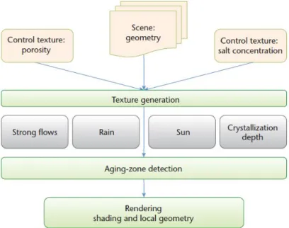
Mérillou et al. [MGGM12] presented another method to simulate the salt deterioration of materials. This process is illustrated in Fig.2.6in a schematic manner, which is essen-tially based on geometry, though it generates textures on-the-fly featuring damages on objects in 3D scenes. Salt decay originates different damage patterns (see Fig.2.7) and behaviors, which depending on three main external conditions [MGGM12]: (i) exposure to, for example, to rain or sunlight; (ii) height (i.e., capillary rise from the ground); and (iii) architectural features (e.g., sculptures, facades, or windows). In general, damage has much to do with three physical material features: mechanical strength, porosity, and salt content. Deterioration occurs because materials are porous, allowing for water (with salt) seepage, so that salt ends up remaining in such materials after evaporation

(27)

caused by the sunlight, a phenomenon called crystallization, as illustrated in Fig.2.8.

IEEE Computer Graphics and Applications 45

The Crystallization Depth

Crystallization results from competition between evaporation (from the sun’s heat) and water loaded with salts (brine) in the porous network of a material through the processes of wetting or capillary rise (see Figure 3). When the brine comes in faster than it evaporates, it seeps through the material’s surface and causes crystallization, moving from inside the pores to the material’s outer surface. If it evaporates faster than it comes in, crystallization occurs inside the material within a few millimeters of its outer surface.

The physical equations driving this competition can help us assess its computability in the context of a physically inspired model that’s suitable for im-age synthesis. (A full derivation of the model ap-pears elsewhere.3_{) Here, we focus on basic physical}

rules to illustrate the necessary parameters’ origins.

Evaporation. Crystallization depth can be

theoreti-cally expressed by Fick’s first law. This law gives the vapor diffusion flux J (in our case, this concerns evaporation) through the thickness of a porous medium, expressed as a pressure difference:

J₌D(Ps−Pa)( /ρ T)

δ

R _, ₍₁₎

where D is the diffusion coefficient, ρ is the vapor’s density, T is the temperature, and R is the gas constant. Ps is the pressure at the crystallization

depth δ; Pa is the pressure outside the affected

object.

JFs is the evaporation rate of water in a porous

medium, with Fs being the proportion of the area

covered by the open porosity that contributes to evaporation.

Capillary migration. Poiseuille’s law expresses a

rela-tionship between the volume V of liquid crossing a pore of 1 cm2_{per unit time t and the gradient of}

pressure P at its ends: ∆ ∆ ∆ V t R P L =π η 4 8 . , (2) (a) (b) (c) (d) (e) (f)

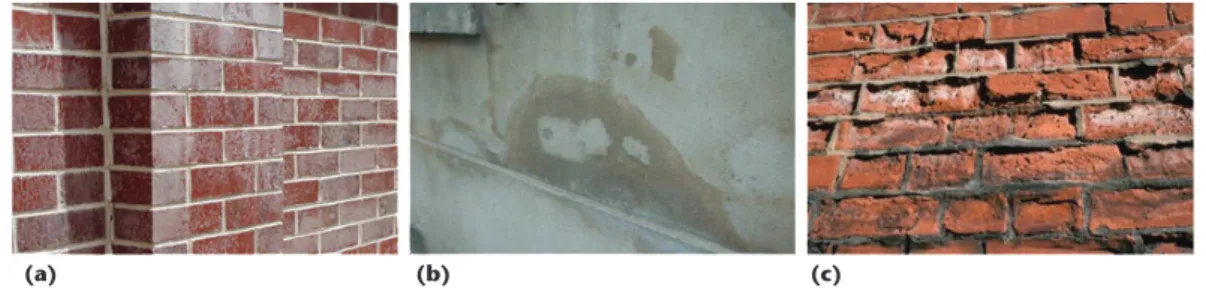
Figure 1. Salt decay effects. (a) Thin efflorescence on a brick wall. (b) Thin efflorescence on a homogeneously cemented wall. (c) Crystallization damage from inside the material near the surface. (d) Another example of crystallization damage. (e) Salt decay on the mortar between low-porosity stone. (f) Salt decay on an ancient painting.

Control texture: porosity

Scene:

geometry _{Control texture:}

salt concentration

Texture generation

Rain

Strong flows Sun Crystallization

depth

Aging-zone detection

Rendering shading and local geometry

Figure 2. Our model for simulating aging due to salt decay. On the basis of intuitive descriptions of material characteristics, we build textures that reflect the effects of strong liquid flows, rain, the sun, and the crystallization depth.

Figure 2.8: Salt decay effects: (a) thin efflorescence on a brick wall; (b) thin efflorescence on a cemented wall; (c) crystallization damage from inside the material near the surface. Source: Merillou et

al. [MGGM12].

2.4 Computational Image Aging

Using only textures and photographs is another method for building aging. As can be seen in this section, photographs and textures, although not being the most realistic way to reproduce aging phenomena, they can reproduce some plausible results in a large scale using low computational resources.

In this area it is very common to find a wide range of systems to capture data from a model or a simple object, from which one compiles all the information and creates pixel values, or even create texture patches, that are then applied to another model that is correlated to those through one or more control variables. Those variables can be: how much aged the model is, the weathering degree and it even can be the propri-ety of the material, e.g. if is stone, rock or marble, and the shape of the model, e.g. the curvature or orientation [BLR+₁₁_{]. Based on this aging method based on textures,} many researchers, like Miller [Mil94] and Hsu and Wong [HW95] started to develop some techniques. Miller [Mil94], started applying ambient occlusion to those pixel values cre-ated in the systems explained before, and Hsu and Wong in [HW95] started using surface exposure, and that happened because has also been found to be highly correlated with weathering concentration.

Wang et al. [WTL+₀₆_{] presented a technique where he captures examples of} differ-ent “degrees” of weathering of a single effect in a single image. The objective in this research is, from this examples, create the basis of an “appearance manifold”. This basis is used to approximate subspace of weathered surface appearance for a material. Many other researchers started from this idea, like the Xue et al. [KRFB06], where he started from where the Wang et al. [WTL+₀₆_{] ended and developed a interactive} edit-ing of weather effects, startedit-ing to transfer from one picture to another those effects. However there are some capture techniques to obtain aged appearance that are a little more sophisticated [WLL+₀₉_{]. In there it is possible to find techniques implemented by} Koudelka [Kou04], Gu et al. [GTR+₀₆_{] and Sun et al. [}_SSR+₀₆_{] that capture time-varying} reflection data for flat surfaces.

(28)

Other researcheers, studied how weathering affects the aging perception using the flow phenomena. Bosch et al. [BLR+₁₁_{], is an example of those researchers and used the} flow phenomena, were instead of modeling the environment, he used a technique where simulate the weathering decay, using only textures. This technique takes a wide range of photos taken to real examples, applies a algorithm to get the flow data and associates it some parameters. With that algorithm he can retrieve the degree map, flow deflec-tion model, gradient-based vector field, and without defecdeflec-tion texture. After that the results are assimilated to the program that is able to generate some new models based on the input photos and apply the results to the computer model. With this method a the program can use photos to generate realistic flow phenomena rather than using photos directly for texture.

As we can see, there is an example from real life in Fig. 2.9, then the processing method, Fig. 2.10and then the final results in Fig. 2.11.

Figure 2.9: Example from real life where we can see the flow phenomena. Source: Bosch et al [BLR+₁₁_].

(29)

Figure 2.11: Some examples from the final result. Source: Bosch et al [BLR+₁₁_].

2.5 Concluding Remarks

Most real world objects are subject to aggressive environmental conditions. These ob-jects react to these conditions by changes in their appearance, which is usually called weathering. This chapter has reviewed the relevant literature concerning building aging algorithms and techniques, with a focus on weathering phenomena, including pollution and salt decay. In the next chapter, we will introduce our algorithm for 3D building aging, which essentially is a procedural technique based on textures.

(30)

(31)

Chapter 3

Noisy Texture-Based Aging Algorithm for Buildings

In this chapter, we detail our texture-based aging algorithm for buildings. This algorithm follows a procedural aging technique that builds upon textures featuring the degradation of building walls, so that it is applicable to one or more city buildings.

3.1 Introduction

As shown in the previous chapter, there are mainly two methods of dealing with ag-ing of materials: geometry-based and texture-based. By changag-ing geometry, we get in principle more realistic degradation effects than using only textures, because of the in-herent and sound representation of depth. However, texture-based methods are much less time-consuming, because their computations are exclusively to handle textures on GPU. Even, when one uses empirical formulas to get more plausible effects of wall dam-ages, they do not represent the physical laws underlying the processes of crystallization and pollution.

The method described in this chapter does not use geometry degradation, so that only textures are used on the unchanged geometry. More specifically, our method lever-ages a set of imlever-ages and textures previously selected and treated, from which we can observe the evolution of aging happening in real time. This algorithm makes usage of shader programming in order to benefit of the GPU power available on most commodity computers (e.g., laptops, desktops, and other compute devices) available today. Our algorithm comprises the following five steps:

• Initialize all resources (textures). • Bind all the textures.

• Aging evolution over time. • Blend all the textures. • Bump mapping.

The first three steps run on CPU side, while the last two are executed on GPU side using shaders. These steps are detailed in the following sections.

(32)

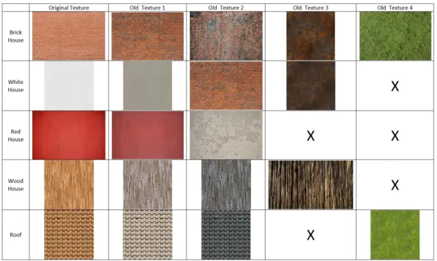
Figure 3.1: Table with all textures used in the thesis tests. The ”X”’s indicates that there are no texture in that category.

(a) (b) (c)

Figure 3.2: (a) Is a normal/height map from the Brick house original texture. (b) Is a normal/height map from the Roof original texture. (c) Is a normal/height map from the Wood house old texture number 3.

3.2 Initialize all resources

As said before first we need to have some pre required files in order to run the algorithm. These files are the textures and their Normal Maps (height map) of each wall of the build, and for the roof as well. As you can see in the table 3.1bellow, these are the pre textures used in this thesis and in the image3.2some examples of the normal maps used for each of the houses. The textures represent the state of the wall (original and degraded state), and the masks represents the effect of degradation that will have. Further on, it will be explained the importance of the masks, and the original and degraded textures.

Now lets take an overview step by step through the algorithm. Before even start it is needed to have a previous study done and a set of textures, for the walls and for the roof, arranged in order to have some visual effect working on. This set of textures can be nothing more nothing else like the ones showed in the table 3.1. After the set is

(33)

arranged all conditions are reunited to start the algorithm.

The first step in this algorithm occurs even before the algorithm is running in real time, executing one time only. In this step the main focus is to initialize all resources, that will be needed algorithm

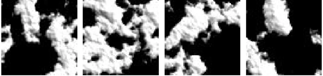
First of all what we need to do is generate some masks. Masks are nothing more than textures shaded in black and white like the ones in Fig. 3.3, and those masks in com-puter graphics have the purpose to blend one texture into another, like for example the black pixels are represented by the texture ”A” and then the white pixels repre-sented by the texture ”B”, creating a new mixed texture with the oldest ones, as we can see further on in Fig. 3.9. To help creating this mask textures, a new library was imported called libnoise. This libnoise library is used to generate coherent noise, a type of smoothly-changing noise, this library is often used to generate perlin noise, that is what is going to be used to creating those masks, it can also generate ridged multifractal noise, and other types of coherent-noise. To get started on this libnoise algorithm first of all it is needed to identify some initial values, the most significant values to take in consideration are seed, texture name, octaves, frequency, gradient, Xcoordinates and Ycoordinates.

The seed value is important because it determines the randomness of the mask, differ-ent values will generate always differdiffer-ent textures/masks, changing this value for each mask is important because if not, all the walls will have the same mask applied to it, giving the same aging effect, in Fig. 3.3 we can see some masks with different seed values. Texture name is a obvious value that will determine what is the mask that is re-lated to particular wall. Ocataves is also an important value, because it determines how strong the frequencies will be 3.4. Frequency is the number of cycles per unit length that the algorithm function outputs, as we can see in Fig. 3.5. Gradient is a important value because it determines the colors in the texture taking in consideration the values from the output, e.g. in a scale from 0 to 100, values between 0 and 30 are blue, repre-senting water, 30 to 40 yellow, reprerepre-senting sand, 40 to 60 green, reprerepre-senting forests, 60 to 90 brown, representing mountains, and 90 to 100 white, representing snow, now since the masks are black and white the algorithm will only consider 2 gradients black and white, split by a small gap represented in a gray color, and the gap will be the interval that determinate the amount of black and white in the mask. And last but not the least, the Xcoordinates and the Ycoordinates, this will determine two things: the amount of ”frequency” that is caught on the texture and where to caught, as Fig. 3.6

shows determining where and how much. This as two advantages, first it is possible to create some randomness selecting always different pieces from the 2D space. And the second is the possibility to select the amount of frequency, as it is possible to see in Fig. 3.6, e.g. if is desired a more square texture/mask or a more stretched one. As explained before the seed value was changed for each face because we always want a different mask for a different wall and a different mask each time we run the procedural build aging algorithm. The size value of the masks was changed to a small value because,

(34)

Figure 3.3: This figure shows a set of masks generated by libnoise using a different seed values.

Figure 3.4: This image shows six octaves combined to form Perlin Noise. Source [Jas]

the amount of pixels influences the computational performance, the more pixels it has to analyze the heavier is the program, and beside that we need to take in consideration that at least we need to create eight masks for each house and using them in real time calculations, so to get a better performance the size was reduced.

3.3 Bind all the textures

Now that all the initial and pre work is done. The algorithm started to run in real time, and simultaneously between two different platforms, the CPU and the GPU. From this point on, in the CPU side will be treated mostly the processing related with variable changing and texture binding in the GPU side will handle the texture rendering, this technique is called OpenGL Shading Language or GLSL. OpenGL Shading Language is a programming language that has been designed to allow programmers more control over the processing that occurs at vertex processing and fragment processing of the OpenGL pipeline.

In the CPU side the first step is to assemble all the textures to each face of the house and then to the roof. In here it is necessary to bind all the textures that we will work with, e.g. it is necessary to bind four groups of textures, one representing the pristine wall 3.1 ”Original Texture” column , other group is the wall with some aged effects

3.1 ”Old 1/2/3/4 Texture” columns, another group with all the normal maps of those textures 3.2and at last all the mask textures 3.3.

Before going any further lets explain the role that all the four groups will have in this algorithm. First of all, as we already know, a wall starts in his pristine state, where all the materials and components stay without any degradation, those are the base of everything, this set of textures represents the first group of textures, 3.1 ”Original Texture” column.

(35)

(a) (c)

Figure 3.5: (a) Mask with low frequency. (b) Mask with high frequency. As it is possible to see, the amount of spikes in the height values are more frequent.

The second set of textures represents two different kinds of aged textures, those tex-tures will be the ones that will be blended into the original one. First of all we have textures that are the same as the original one, but have some work on it to look aged or even degraded, and in the second hand we have textures that nothing have to do with the original texture but have some aged effect to give more realism to the aging process like as we can see in Fig. 3.1, ”Old 3/4 Texture” columns.

The third set of textures is the normal map from all the pristine and aged textures, that is nothing more than a texture that represents a height map. The normal maps are used in the technique called bump mapping, this technique was chosen because in a large scale 3D environment or in a large scale city, it is desired to not change the geometry, or change it the minimum possible, because the more we change the more vertex we will have, and with it more vertex to render more heavier the computational level is. So to be able to scale this algorithm to an ever larger scale, the bump mapping was implemented. The bump mapping is a technique that for each object pixel that is being rendered, it is applied a perturbation in its normal surface, based on the normal map (height map). As Fig. 3.2show there is how a normal map looks like, and in Fig. 3.7

how it looks like applied to an object.

At last, the fourth set of textures are the mask textures. This set of textures repre-sents all the masks that will be used in this algorithm, as explained before this set of images are created based only in two colors, black and white, this is because we want a more strait simple and contrasted image possible. To have a very contrasted image is important because the masks in computational graphics have a simple task, one color represents one texture and another color represents another texture. In this partic-ular case the black pixels will represent the original texture and the white ones will represent the aged texture.

3.4 Aging Evolution

Now that all the textures from all faces are being sent from the CPU to the GPU side, on the CPU side it is needed to do only one more thing, to go updating the variables so that the aging process can evolve. At each needed interaction, tree values are changed,

(36)

(a)

(b) (c)

Figure 3.6: (a) In here the rectangle represents the mask area, where the bottom-left coordinates are (2,1) and its upper-right coordinates are (6,5). Source [Jas]. (b) In here it is possible to see an example

of the same quad as image ”a”. (c) In this image we can see the same mask but now although the representation still a square, the bound limit is stretched in the ”X” axis.

Figure 3.7: This is how the bump mapping looks like if we force a light pass near the wall. In a 2D image, we can create a sense of relief, by just distorting the incident light in the texture with the weight map.

the first and the most important one is the aging value, this value is the one that will define in which stage of degradation, the house is. Then the second variable that we will talk about is called ’bright’, and this variable has this name because this is the one that will determine how much black and how much white the mask will have, in other words it is right to say the amount of brightness that the mask will have. And for last, the variable that will determine the amount of relief done by the bump mapping, if it

(37)

is more or less notorious.

3.5 Blend all the textures and bump mapping

Now is where all the action is taken to the GPU side, in here is where all the textures are rendered, blended and the bump mapping comes to live.

As we saw before all the code from the GPU side will be executed under the GLSL (OpenGL Shader Language) technology. This technology mainly works with two pro-grammable files, one called ”vertex shader” and other called ”fragment shader”, each one this files has a very specific role in the render part. The ”vertex shader” is respon-sible to execute its code for each vertex the program will draw, e.g. if I want to draw a square the program will execute the ”vertex shader” four times. Then we have one last file, the ”fragment shader” and this probably is the most important one for this algorithm because it will be executed for each pixel/fragment that we want to draw. In the vertex shader, all the code stay as default, since all the aging process is based only in visualization, texture work and bump mapping techniques, all the developed code are in the fragment/pixel shader.

The fragment/pixel shader holds the core code responsible to represent and simulate the aging process. In this shader the first thing to do is to store all the variables sent from the CPU side, those variables are essentially the light position and all the four groups of textures, examinated before. The first step of the algorithm is to blend all the textures to one face, taking in consideration some rules and order. The first blend process is to mix the original one, with itself, just giving a dark/old perspective to it. Then, in the next process, the texture resulted from that mix will be blended with the first old texture representing some aging effect, taking in consideration one mask. In here the 1st texture will appear in the black pixels of the mask and the first old texture in the white pixels. Then we repeat this last process for each bad texture, taking in consideration always the last texture resulted from the mix. In the next step we will do the same kind of mix but now with the normal/height maps, for a precise relief in the texture wall (bump mapping). And at last, for each pixel in the screen, taking in consideration the normal/height texture resulted from the mix, the fragment shader will apply the bump mapping technique.

3.6 Algorithm applied in a real test

3.6.1 Initialize all resources

Starting from the beginning lets take a look in the init function, this function only runs one time as the program starts. For a better understanding of this code lets split it in

(38)

groups. So in the first group the algorithm will load all the vertex and the fragment/pixel shaders to the GPU side, this is an important step because all of this files hold the code that will run in the GPU side, for each single file. As can be seen, it was created a vertex shader and a fragment/pixel shader for each group of textures, or in other words each surface that need to be worked. This decision was made to give the programmer a better and unique control of each face.

1 \ * I n i t F u n c t i o n * \ 2 3 void I n i t ( ) { 4 5 \ * 1 s t Group * \ 6 s h a d e r T e x t u r e F l o o r = s e t S h a d e r s ( ” Shaders / s h a d e r s T e x t u r e s C h a o . v e r t ” , ” Shaders / s h a d e r s T e x t u r e s C h a o . f r a g ” , s h a d e r T e x t u r e F l o o r ) ; 7 s h a d e r T e x t u r e F S = s e t S h a d e r s ( ” Shaders / s h a d e r s T e x t u r e s F S . v e r t ” , ” Shaders / s h a d e r s T e x t u r e s F S . f r a g ” , s h a d e r T e x t u r e F S ) ;

8 shaderTextureFO = s e t S h a d e r s ( ” Shaders / s h a d e r s T e x t u r e s F O . v e r t ” , ” Shaders / s h a d e r s T e x t u r e s F O . f r a g ” , shaderTextureFO ) ;

9 shaderTextureFN = s e t S h a d e r s ( ” Shaders / s h a d e r s T e x t u r e s F N . v e r t ” , ” Shaders / s h a d e r s T e x t u r e s F N . f r a g ” , shaderTextureFN ) ;

10 shaderTextureFE = s e t S h a d e r s ( ” Shaders / s h a d e r s T e x t u r e s F E . v e r t ” , ” Shaders / s h a d e r s T e x t u r e s F E . f r a g ” , shaderTextureFE ) ; 11 sh a de r Te x tu re R oo f = s e t S h a d e r s ( ” Shaders / s h a d e r s T e x t u r e s R o o f . v e r t ” , ” Shaders / s h a d e r s T e x t u r e s R o o f . f r a g ” , s ha d er T ex tu r eR o of ) ; 12 s h a d e r T e x t u r e A c e s s = s e t S h a d e r s ( ” Shaders / s h a d e r s T e x t u r e s A c e s s . v e r t ” , ” Shaders / s h a d e r s T e x t u r e s A c e s s . f r a g ” , s h a d e r T e x t u r e A c e s s ) ; 13 14 ( . . . )

Then in the second group, is where all the ambient light is applied to each shader, what means to each face. In here the same logic, from the group before, is applied. As all sides have their own light, so the customization and the independence are a bonus. With that we can have some custom features, like a specific light that influences only one wall, or a light with a different color and cause this is the light used in the bump mapping, in here it is possible to define too how much effect the bump mapping will have, using the variable ”val relief”. In this group inside the init lights defined values such ambient color, screen resolution, light color and light position.

1 \ * I n i t F u n c t i o n * \ 2 3 void I n i t ( ) { 4 5 ( . . . ) 6 7 \ * 2nd Group * \ 8 I n i t _ L i g h t ( s h a d e r T e x t u r e F l o o r , 0 . 5 ) ; 9 I n i t _ L i g h t ( shaderTextureFS , v a l _ r e l i e f _ F ) ; 10 I n i t _ L i g h t ( shaderTextureFO , v a l _ r e l i e f _ F ) ;

(39)

11 I n i t _ L i g h t ( shaderTextureFN , v a l _ r e l i e f _ F ) ; 12 I n i t _ L i g h t ( shaderTextureFE , v a l _ r e l i e f _ F ) ; 13 I n i t _ L i g h t ( shaderTextureRoof , v a l _ r e l i e f _ R ) ; 14 I n i t _ L i g h t ( sh ad er Tex tu reA ce ss , v a l _ r e l i e f _ A ) ; 15 16 ( . . . )

In the third group is where all the pre worked textures are loaded to the program. In here we can find the original textures and its height/normal map.

1 \ * I n i t F u n c t i o n * \ 2 3 void I n i t ( ) { 4 5 ( . . . ) 6 7 \ * 3 rd Group * \ 8 t e x _ I D _ F l o o r = LoadBMPPNG_Texture ( ” T e x t u r a s / f l o o r T . png” ) ; 9 norm_ID_Floor = LoadBMPPNG_Texture ( ” Normals / f l o o r N . png” ) ; 10

11 t e x _ I D _ F S = LoadBMPPNG_Texture ( ” T e x t u r a s / wallT .bmp” ) ; 12 norm_ID_FS = LoadBMPPNG_Texture ( ” Normals / wallN . png” ) ; 13

14 tex_ID_FO = LoadBMPPNG_Texture ( ” T e x t u r a s / wallT .bmp” ) ; 15 norm_ID_FO = LoadBMPPNG_Texture ( ” Normals / wallN . png” ) ; 16

17 tex_ID_FN = LoadBMPPNG_Texture ( ” T e x t u r a s / wallT .bmp” ) ; 18 norm_ID_FN = LoadBMPPNG_Texture ( ” Normals / wallN . png” ) ; 19

20 t e x _ I D _ F E = LoadBMPPNG_Texture ( ” T e x t u r a s / wallT .bmp” ) ; 21 norm_ID_FE = LoadBMPPNG_Texture ( ” Normals / wallN . png” ) ; 22

23 t e x _ I D _ R o o f = LoadBMPPNG_Texture ( ” T e x t u r a s / r o o f T .bmp” ) ; 24 norm_ID_Roof = LoadBMPPNG_Texture ( ” Normals / roofN . png” ) ; 25

26 t e x _ I D _ D o o r = LoadBMPPNG_Texture ( ” T e x t u r a s / doorT . png” ) ; 27 norm_ID_Door = LoadBMPPNG_Texture ( ” Normals / doorN . png” ) ; 28

29 tex_ID_W1 = LoadBMPPNG_Texture ( ” T e x t u r a s /windowT . png” ) ; 30 norm_ID_W1 = LoadBMPPNG_Texture ( ” Normals /windowN . png” ) ; 31

32 ( . . . )

At last, in the final group of the init function, we can find the mask initialization. In here is where the masks are created for each face and for each bad/old texture that will be applied to each face, as presented before all this work is done with the help of libnoise library. Since the start, all the masks are black, because we want a pristine house and not already a old one. Many of these input values don’t do much, but lets

(40)

take a overview on them anyway, and what each variable should do in this function. For this function we can find eleven variables:

1 \ * Create Mask F u n c t i o n * \

2 void Create_bmp_mask ( i n t Seed , i n t C o n t r a s t , i n t B r i g h t n e s s , s t d : : s t r i n g Name,

i n t Octaves , f l o a t Frequency , f l o a t max_value , f l o a t H i g h _ L i m i t , f l o a t

X_Frame , f l o a t Y_Frame , i n t I D ) { . . . } 3 4 \ * I n i t F u n c t i o n * \ 5 6 void I n i t ( ) { 7 8 ( . . . ) 9 10 \ * 4 th Group * \

11 Create_bmp_mask ( 0 , 3 . 0 , 2 . 0 , ” Masks /mask_FS_O2 .bmp” , 12 , 1 . 5 , 2 . 0 1 , 0 . 2 , 50 , 5 0 . 0 , 1 ) ;

12 Create_bmp_mask ( 0 , 3 . 0 , 2 . 0 , ” Masks /mask_FS_O .bmp” , 12 , 1 . 5 , 2 . 0 1 , 0 . 2 , 50 , 5 0 . 0 , 1 ) ;

13

14 Create_bmp_mask ( 0 , 3 . 0 , 2 . 0 , ” Masks /mask_FO_O2 .bmp” , 12 , 1 . 5 , 2 . 0 1 , 0 . 2 , 50 , 5 0 . 0 , 1 ) ;

15 Create_bmp_mask ( 0 , 3 . 0 , 2 . 0 , ” Masks /mask_FO_O .bmp” , 12 , 1 . 5 , 2 . 0 1 , 0 . 2 , 50 , 5 0 . 0 , 1 ) ;

16

17 Create_bmp_mask ( 0 , 3 . 0 , 2 . 0 , ” Masks /mask_FN_O2 .bmp” , 12 , 1 . 5 , 2 . 0 1 , 0 . 2 , 50 , 5 0 . 0 , 1 ) ;

18 Create_bmp_mask ( 0 , 3 . 0 , 2 . 0 , ” Masks /mask_FN_O .bmp” , 12 , 1 . 5 , 2 . 0 1 , 0 . 2 , 50 , 5 0 . 0 , 1 ) ;

19

20 Create_bmp_mask ( 0 , 3 . 0 , 2 . 0 , ” Masks /mask_FE_O2 .bmp” , 12 , 1 . 5 , 2 . 0 1 , 0 . 2 , 50 , 5 0 . 0 , 1 ) ;

21 Create_bmp_mask ( 0 , 3 . 0 , 2 . 0 , ” Masks /mask_FE_O .bmp” , 12 , 1 . 5 , 2 . 0 1 , 0 . 2 , 50 , 5 0 . 0 , 1 ) ;

22

23 tex_ID_F_B1 = LoadBMPPNG_Texture ( ” T e x t u r a s / wallOT .bmp” ) ; 24 tex_ID_F_B2 = LoadBMPPNG_Texture ( ” T e x t u r a s / wallDT .bmp” ) ; 25 tex_ID_F_B1_N = LoadBMPPNG_Texture ( ” Normals / wallON . png” ) ; 26 tex_ID_F_B2_N = LoadBMPPNG_Texture ( ” Normals / wallDN . png” ) ; 27

28 ( . . . )

1. Seed - this variable has the purpose to set the seed for the libnoise algorithm. For each different seed it is possible to generate a different mask, this happens because the seed value determines how the perlin noise is generated.

2. Contrast - the contrast is the value that will determine how much contrast the image will have. This is important because in a white and black texture we do not

(41)

want shades of gray.

3. Brightness - as the contrast the brightness have the same function, to eliminate some gray shades.

4. Name - in here as the name says, is where the texture name is passed, this allow us to specify the mask that we want.

5. Octaves - octaves is the number that define how much times the perlin-noise function is called. The perlin noise i sum of several coherent-noise functions with ever-increasing frequencies and ever-decreasing amplitudes. An octave is one of these functions, the number of octaves determines how much functions will occur. As we want more variety the number is increased.

6. Frequency - is the variable that determinate how much irregular the noise can be. If the frequency is high we can find much more white and black spots, and if it is low we will find a more smooth transition between the black and white color. For this aging process we want a smooth transition so the value is quite low.

7. High Limit - defines the maximum frequency possible, in the perlin noise.

8. Interval - The interval defines how high the white gradient starts. We want a value right above the maximum frequency possible because, at the start, we want a black mask/texture. Over time that black texture will originating some white spots. This can be possible lowering this interval.

9. X Frame - The X frame determines how wide the image will be. For example if the X frame is 2 and Y frame is 1 it will be wider than long, and if the X frame is set to 1 and Y frame equals 1, we have a perfect square. This is an important feature because a wider mask is more suitable for textures that have wight objects e.g. brick house, and a long mask for long objects e.g. a wood house that have the wood placed vertically.

10. Y Frame - The same as X frame but for the Y axis.

11. ID - this ID represents the group of textures that will be influenced by some aging process, as an example for this thesis all the textures were arranged in 3 groups. One for faces, another for the roof and another for doors and windows. This allows to have some different aging process for those groups.

3.6.2 Bind all the textures and Aging Evolution Controller

In the next step all the code will be running in real time. And since all the following code runs in practically at the same time we can assume ”Bind all the textures and Aging Evolution Controller” steps as one.

(42)

So in the first step the algorithm binds to each face all the textures, all the height/nor-mal maps and finally all the masks. Then if the old value was changed the algorithm triggers a new mask generation, lets study that in a second. This old value is the most important value for this algorithm because it is the one that will define how old the ob-ject is. As explained before, because all the obob-jects have a separated aging processes we could define different aging values for each object, in this case for each wall, but since that is just a customization option all the walls in this thesis will be affected by the same old value. Resuming back to the process, if the ”old value” is changed then the function is triggered and with it some variables need to be passed to the function ”getOld”: 1 \ * Each Object F u n c t i o n * \ 2 3 void FaceSouth ( ) { 4 5 glUseProgram ( s h a d e r T e x t u r e F S ) ; 6 GLuint F S _ t e x t u r e = g l G e t U n i f o r m L o c a t i o n ( shaderTextureFS , ” F S _ t e x t u r e ” ) ; 7 g l U n i f o r m 1 i ( F S _ t e x t u r e , 0 ) ;

8 GLuint FS_NormMp = g l G e t U n i f o r m L o c a t i o n ( shaderTextureFS , ” FS_normals ” ) ; 9 g l U n i f o r m 1 i ( FS_NormMp , 1 ) ;

10

11 GLuint t e x t u r e _ B 1 = g l G e t U n i f o r m L o c a t i o n ( shaderTextureFS , ” Texture_B1 ” ) ; 12 g l U n i f o r m 1 i ( texture_B1 , 2 ) ;

13 GLuint Texture_B1_N = g l G e t U n i f o r m L o c a t i o n ( shaderTextureFS , ” Texture_B1_N ” ) ; 14 g l U n i f o r m 1 i ( Texture_B1_N , 3 ) ;

15

16 GLuint t e x t u r e _ B 2 = g l G e t U n i f o r m L o c a t i o n ( shaderTextureFS , ” Texture_B2 ” ) ; 17 g l U n i f o r m 1 i ( texture_B2 , 4 ) ;

18 GLuint texture_B2_N = g l G e t U n i f o r m L o c a t i o n ( shaderTextureFS , ” Texture_B2_N ” ) ; 19 g l U n i f o r m 1 i ( texture_B2_N , 5 ) ;

20

21 GLuint Texture_M_O = g l G e t U n i f o r m L o c a t i o n ( shaderTextureFS , ”Texture_M_O” ) ; 22 g l U n i f o r m 1 i ( Texture_M_O , 6 ) ;

23 GLuint Texture_M_O2 = g l G e t U n i f o r m L o c a t i o n ( shaderTextureFS , ” Texture_M_O2 ” ) ; 24 g l U n i f o r m 1 i ( Texture_M_O2 , 7 ) ;

25

26 get_Old_F ( shaderTextureFS , ” Masks /mask_FS_O2 .bmp” , 0 , 0 ) ; 27 get_Old_F ( shaderTextureFS , ” Masks /mask_FS_O .bmp” , 0 , 0 ) ; 28

29 ( . . . ) 30

31 void get_Old_F ( GLuint shader_Program , s t d : : s t r i n g name , i n t id , i n t v a l _ i d ) {

. . . }

1. Shader Program - this variable represents the shader that will work with a specific mask, as we saw before different shaders were created for different walls.

(43)

2. Mask name - as the variable name says, this represents the mask that we will re-generate.

3. ID - this ID represents the group of textures that will be influenced by some aging process.

4. Seed(val id) - this variable is the one that represents the seed value for the libnoise algorithm. This is useful because different masks could have different seed values.

After the function receives all variables the first step activates the corresponding shader for that face. Then the ”old value” is updated and sent to the shader (GPU side), this happens because as we are going to see ahead, this value will influence how the textures will be processed on the GPU side. Then only two verification’s need to be done, and the conditions that are verified are if the object already reached the maximum old level desired, and what kind of mask we are talking about. The old level desired is an important value because it will determine how old we want an object, forcing that same object not going older than what we want. The mask name is also verified by the simple fact that different groups or different masks could have different transformations. In this example we can find that we have two groups of masks, one is responsible for one aging process and the other for another process, as an e.g. in a house with a painted wall, the first aging process could be the ink changing or losing color, and the second aging process could be the ink falling, causing the wall to lose its ink layer. If all the conditions became to be false, then in the next step the function just loads the mask created before with no changes, if not and all the conditions are true, the function in the next step will resume the aging process by changing the brightness. As explained before, this brightness will help give to the object a more dark appearance, highlighting all its relief and aging effects, and will help determining how much white and black the mask will have. Now that we have the two new values, the ”old value” that represents how old the object is and the ”bright value”, that represents how much white will be in the mask, we can start to re-generate the mask. Calling the function to re-generate the mask, have the same process, explained before, that was used on the init function, the only difference is the bright value. Since this value is the one that represents where the black ends and the white starts, as it is smaller the greater is the amount of white in the mask 3.8. Now that the mask is regenerated, only left to load again the mask to the CPU memory, to bind it to the walls. After that, all the textures are now bind to the respective object, letting all the work from the CPU side done.

1 \ * Old Faces F u n c t i o n * \ 2

3 void get_Old_F ( GLuint shader_Program , s t d : : s t r i n g name , i n t id , i n t v a l _ i d ) { 4 glUseProgram ( shader_Program ) ;

5 G L f l o a t v_O = g l G e t U n i f o r m L o c a t i o n ( shader_Program , ” v a l u e _ o l d ” ) ; 6

7 i f ( v a l _ O l d [ i d ] > 0 . 0 )

(44)

(a)

(b)

Figure 3.8: This figure shows the mask result in (a) of an unchanged ”bright value”. And in (b) it is possible to see the result of the mask when the ”bright value” is at half.

9 v a l _ O l d [ i d ] −= 0.001; 10 } 11 12 f l o a t v a l = ( v a l _ O l d [ i d ] − ( 0 ) ) / (1.8 − ( 0 ) ) ; 13 v a l −= 1; 14 v a l = abs ( v a l ) ; 15 g l U n i f o r m 1 f ( v_O , v a l ) ; 16 17 i f ( v a l _ O l d [ i d ] < 0 && b r i g h t [ i d ] >= −0.1) 18 {

19 i f ( ( name == ” Masks /mask_FS_O .bmp” || name == ” Masks /mask_FO_O .bmp” || name

== ” Masks /mask_FN_O .bmp” || name == ” Masks /mask_FE_O .bmp” ) && b r i g h t [ i d ] >= −0.1 && flag_avanca_env == 0)

20 {

21 b r i g h t [ i d ] −= 0.004;

22 Create_bmp_mask ( v a l _ i d , 2 . 0 , 2 . 0 , name , 12 , 3 , 2 . 0 1 , 0 . 2 , 1 . 0 , 1 . 0 , i d ) ; 23 tex_ID_F_M_O = LoadBMPPNG_Texture ( name ) ;

24 i f ( b r i g h t [ i d ] <= −0.09 ) 25 { 26 b r i g h t [ 0 ] = 1 . 2 ; 27 f l a g _ a v a n c a _ e n v = 1 ; 28 } 29 } 30 e l s e 31 {

(45)

name == ” Masks /mask_FN_O2 .bmp” || name == ” Masks /mask_FE_O2 .bmp” ) && b r i g h t [ i d ] > 0 . 3 && f l a g _ a v a n c a _ e n v == 1 ) 33 { 34 b r i g h t [ i d ] −= 0.004; 35 Create_bmp_mask ( v a l _ i d , 2 . 0 , 2 . 0 , name , 12 , 2 , 2 . 0 1 , 0 . 2 , 2 . 0 , 2 . 0 , i d ) ;

36 tex_ID_F_M_O2 = LoadBMPPNG_Texture ( name ) ; 37 i f ( b r i g h t [ i d ] <= 0 . 3 ) 38 { 39 b r i g h t [ 0 ] = −1.8; 40 } 41 } 42 e l s e 43 {

44 i f ( ( name == ” Masks /mask_FS_O2 .bmp” || name == ” Masks /mask_FO_O2 .bmp”

|| name == ” Masks /mask_FN_O2 .bmp” || name == ” Masks /mask_FE_O2 .bmp” ) )

45 {

46 tex_ID_F_M_O2 = LoadBMPPNG_Texture ( name ) ;

47 }

48 i f ( ( name == ” Masks /mask_FS_O .bmp” || name == ” Masks /mask_FO_O .bmp” ||

name == ” Masks /mask_FN_O .bmp” || name == ” Masks /mask_FE_O .bmp” ) )

49 {

50 tex_ID_F_M_O = LoadBMPPNG_Texture ( name ) ;

51 } 52 } 53 } 54 } 55 e l s e 56 {

57 i f ( ( name == ” Masks /mask_FS_O2 .bmp” || name == ” Masks /mask_FO_O2 .bmp” ||

name == ” Masks /mask_FN_O2 .bmp” || name == ” Masks /mask_FE_O2 .bmp” ) )

58 {

59 tex_ID_F_M_O2 = LoadBMPPNG_Texture ( name ) ;

60 }

61 i f ( ( name == ” Masks /mask_FS_O .bmp” || name == ” Masks /mask_FO_O .bmp” || name

== ” Masks /mask_FN_O .bmp” || name == ” Masks /mask_FE_O .bmp” ) )

62 {

63 tex_ID_F_M_O = LoadBMPPNG_Texture ( name ) ;

64 } 65 } 66 67 68 i f ( v a l _ O l d [ i d ] <= 0 . 2 && v a l _ r e l e v o _ F >−0.2) 69 { 70 v a l _ r e l e v o _ F −= 0.001; 71 } 72 }

(46)

Until now we saw that the program was already doing some important things. In the start it loaded all the textures to memory, create all light sources and create the masks and loaded them. Then after the program start at each iteration it started to bind all textures to each object, and if the old value for that object was changed it triggered the function to re-generate a new mask, if all the condition passed, then the mask was re-generated and then bound to the object. After that all work on the CPU side was done and now it is time from GPU do the work.

3.6.3 Blend all the textures

Since all the work from the CPU side is done, now we will take an overview in the shaders, from the GPU side. Starting from the Vertex shader, since it is the most simple one. For a better understanding, the shader operates on an individual vertex, receiving as input one single vertex, having access to its position, normal vector and texture coordinates. For this aging process we do not want to do any modifications to those attributes, so the code is pretty standard as we can see in the vertex shader code. Now lets take a look in the Fragment shader, which as previously explained is the fragment that will be process pixel by pixel (fragments). In here after all the variables being declared, we start our main function. In this main function the first step is to declare the variables that will be used in the bump mapping such the ”theMatrix” that will hold the light positions and its colors, the next variables are the ones that will represent all the textures, masks and normal/height maps. The variable ”diffuseColor” will be the one that holds the combination of all textures, so let’s start to explain the steps in this mixing. First of all we assigned to the diffuse color the original texture ”FS TEXTURE”, then we mix it with the first bad texture, giving as value to interpolate the ”difuseColor” multiplied by the ”oldvalue”. The reason of this, is to start to give a smooth transition between the two textures and the ”oldvalue” appears here as a starting decay feature. Then in the next step we do the same thing but now for the second bad texture, resulting in one texture with the Original, plus First bad, plus the Second bad textures3.9. Since we only have one bad texture to blend using a mask, we only need one mask, so in the next step we will blend in the ”diffuseColor” the second bad texture, giving as the interpolate value the mask. Since the mask is just black and white, meaning that have the two opposites values available to interpolate, the black will represent the old ”diffuseColor” texture and the white will be representing the second old texture. Now that all the mixed texture is created, we need to do the same with the height/normal map, blending the original normal map with the first bad one, and then blend the result of that mixing with the second bad normal map taking in consideration the mask, allowing that different textures stay with respective relief.

1 \ * Vertex Shader * \ 2

3 void main ( ) 4 {

(47)

(a) (b) (c)

(d)

Figure 3.9: In this figure it is possible to see an example how the mix works. We have the base texture (a), that when mixed with the (b) texture given the mask (c), we got the result (d).

5 gl_TexCoord [ 0 ] = g l _ M u l t i T e x C o o r d 0 ; 6 7 g l _ P o s i t i o n = f t r a n s f o r m ( ) ; 8 9 } 1 \ * Vertex Shader * \ 2 3 void main ( ) 4 {

5 vec3 Sum = vec3 ( 0 . 0 ) ; 6 mat4 t h e M a t r i x ; 7 t h e M a t r i x [ 0 ] = vec4 ( L i g h t P o s , 0 ) ; 8 t h e M a t r i x [ 1 ] = L i g h t C o l o r ; 9 t h e M a t r i x [ 2 ] = vec4 ( L i g h t P o s 2 , 0 ) ; 10 t h e M a t r i x [ 3 ] = L i g h t C o l o r 2 ; 11 12 //RGBA of our d i f f u s e c o l o r

13 vec4 D i f f u s e C o l o r = tex ture 2D ( F S _ t e x t u r e , gl_TexCoord [ 0 ] . s t ) ; 14

15 vec4 t e x e l 0 1 = tex ture 2D ( Texture_B1 , gl_TexCoord [ 0 ] . s t ) ; 16 vec4 t e x e l 0 2 = tex ture 2D ( Texture_B1_N , gl_TexCoord [ 0 ] . s t ) ; 17 vec4 t e x e l 0 3 = tex ture 2D ( Texture_B2 , gl_TexCoord [ 0 ] . s t ) ; 18 vec4 t e x e l 0 4 = tex ture 2D ( Texture_B2_N , gl_TexCoord [ 0 ] . s t ) ; 19 vec4 t e x e l 0 5 = tex ture 2D ( Texture_M_O , gl_TexCoord [ 0 ] . s t ) ; 20 vec4 t e x e l 0 6 = tex ture 2D ( Texture_M_O2 , gl_TexCoord [ 0 ] . s t ) ; 21

22 // D i f f u s e C o l o r = mix ( D i f f u s e C o l o r , texel01 , D i f f u s e C o l o r * v a l u e _ o l d ) ;

23 D i f f u s e C o l o r = mix ( D i f f u s e C o l o r , t e x e l 0 1 , D i f f u s e C o l o r * v a l u e _ o l d ) ; 24 D i f f u s e C o l o r = mix ( D i f f u s e C o l o r , t e x e l 0 3 , D i f f u s e C o l o r * v a l u e _ o l d ) ;

(48)

25 D i f f u s e C o l o r = mix ( D i f f u s e C o l o r , t e x e l 0 3 , t e x e l 0 6 ) ; 26

27 //RGB of our normal map

28 vec4 NormalMapO = text ure 2D ( FS_normals , gl_TexCoord [ 0 ] . s t ) ; 29 //NormalMap . g = 1 . 0 − NormalMap . g ;

30

31 NormalMapO = mix ( NormalMapO , t e x e l 0 4 , D i f f u s e C o l o r * v a l u e _ o l d ) ; 32 vec3 NormalMap = mix ( NormalMapO , t e x e l 0 2 , t e x e l 0 6 ) . rgb ;

33

34 ( . . . ) 35

36 }

3.6.4 Bump Mapping

As the final step we need to do the bump mapping, as explained before the bump mapping is a technique that uses a texture and applies to it a height map, computing it with the ambient light giving us a surface with more detail and relief, simulating the real world. So to achieve this we needed to calculate the delta from light position, then taking in consideration the screen resolution to correct the aspect ration, then we determine the distance from the pixel to the light, after that, the vectors were normalized. At last, all the color was set correctly taking in consideration the light intensity, the ambient color and the attenuation. To conclude, all this calculations are compute to a final result.

1 \ * Fragment Shader * \ 2 3 void main ( ) 4 { 5 6 ( . . . ) 7 8 f o r ( i n t i = 0 ; i < 4 ; i +=2) 9 { 10 //The d e l t a p o s i t i o n of l i g h t

11 vec3 L i g h t D i r = vec3 ( t h e M a t r i x [ i ] . xy − ( gl_FragCoord . xy / Resolution . xy ) , t h e M a t r i x [ i ] . z ) ;

12

13 // C o r r e c t f o r a s p e c t r a t i o

14 L i g h t D i r . x * = R e s o l u t i o n . x / R e s o l u t i o n . y ; 15

16 // Determine d i s t a n c e ( used f o r a t t e n u a t i o n ) BEFORE we normalize our L i g h t D i r

17 f l o a t D = l e n g t h ( L i g h t D i r ) ;

18

Procedural aging techniques of synthetic cities and 3D scenarios