UNIVERSIDADE FEDERAL DO CEARÁ CENTRO DE TENCOLOGIA
DEPARTAMENTO DE ENGENHARIA ELÉTRICA
PROGRAMA DE PÓS-GRADUAÇÃO EM ENGENHARIA ELÉTRICA
FÉLIX EDUARDO MAPURUNGA DE MELO
MODELING AND LINEAR PARAMETER-VARYING IDENTIFICATION OF A TWO-TANK SYSTEM
FÉLIX EDUARDO MAPURUNGA DE MELO
MODELING AND LINEAR PARAMETER-VARYING IDENTIFICATION OF A TWO-TANK SYSTEM
Master’s dissertation presented to the graduate program in Electrical Engineering from Federal University of Ceará as part of the requisites to obtain the Master’s degree in Electrical Engi-neering. Concentration Area: Electrical Energy systems.
Supervisor: Prof. Fabrício Gonzalez Nogueira Co-supervisor: Prof. Arthur P. de Souza Braga
FORTALEZA
Dados Internacionais de Catalogação na Publicação Universidade Federal do Ceará
Biblioteca Universitária
Gerada automaticamente pelo módulo Catalog, mediante os dados fornecidos pelo(a) autor(a)
M485m Melo, Félix Eduardo Mapurunga de.
Modeling and linear parameter-varying identification of a two-tank system / Félix Eduardo Mapurunga de Melo. – 2017.
82 f. : il. color.
Dissertação (mestrado) – Universidade Federal do Ceará, Centro de Tecnologia, Programa de Pós-Graduação em Engenharia Elétrica, Fortaleza, 2017.
Orientação: Prof. Dr. Fabrício Gonzalez Nogueira. Coorientação: Prof. Dr. Arthur Plínio de Souza Braga.
1. Linear com Parâmetros Variantes. 2. Identificação de Sistemas. 3. Sistemas de dois tanques. 4. Modelagem. 5. Máquinas de vetor de suporte. I. Título.
FÉLIX EDUARDO MAPURUNGA DE MELO
MODELING AND LINEAR PARAMETER-VARYING IDENTIFICATION OF A TWO-TANK SYSTEM
Master’s dissertation presented to the graduate program in Electrical Engineering from Federal University of Ceará as part of the requisites to obtain the Master’s degree in Electrical Engi-neering. Concentration Area: Electrical Energy systems.
Approved in July 18, 2017.
EXAMINATION BOARD
Prof. Fabrício Gonzalez Nogueira (Supervisor) Universidade Federal do Ceará
Prof. Arthur P. de Souza Braga (Co-supervisor) Universidade Federal do Ceará
Prof. Wilkley Bezerra Correia Universidade Federal do Ceará
Prof. Guilherme de Alencar Barreto Universidade Federal do Ceará
ACKNOWLEDGEMENTS
I would like to express my gratitude to my supervisor, who introduced me to the theme and have supported me to continue my research path in the system identification field. It was a great pleasure to work with Fabrício during these two years. He provided me not only with his expertise, but also with valuable hints in many aspects of life itself, whose I will carry with me for my entire life as well as his friendship.
I am eternally grateful to my family, who I own everything. Firstly, my not so patient wife, whose love and care always revitalized me every day and filled me with energy to conquer anything in my life. Secondly, my mother that started this journey and have always expressed all the support necessary in my life. Last but not the least, my beloved sister that both of us know we can always count on each other.
Throughout this work I have met many people that have helped me in some way. Then, I would like to thank the professors associated with the GPAR laboratory, which I have spent more time with. The first contribute came from my co-supervisor prof. Arthur, which I have had the chance to learn (and have fun) about computational intelligence. Prof. Bismarck deserves a special thanks for the clarifying talks about systems and predictive control, as well as the development of this work. Profa Laurinda that always made the possible to help me in many issues during this period. Unfortunately, she could not participate in this final stage. Finally, Prof. Wilkley whom I have had fewer time with, but his contributes to this work made the difference. For aforementioned reasons it goes my sincerely thanks.
I would like to thank the examination board, composed by Prof. José Everardo Bessa Maia and Prof. Guilherme de Alencar Barreto, for the time spent in analyzing this work. A special thanks goes to Prof. Everardo, who introduced me to the system identification field and the unmeasurable guidance inspired me to take this path in my life.
If I list all the reasons to be grateful to my friends for everything they have done this section would have more pages than the entire work. I simply do not dare to translate in words the shared moments we have had together. Then, I have chosen to name each one of you in alphabetical order: Adriano, Aluisio, Caio, Clauson, Fábio, Paulo, Magno, René, and Silas. Each one of you know exactly what you have made for me. A special thanks goes to my friend Matheus for kindly revising this text.
ABSTRACT
This work addresses the modeling and the linear parameter-varying (LPV) system identification of a coupled two-tank system (TTS). The system is a multiple input multiple output (MIMO) with two inputs and two outputs. In order to obtain a suitable model for this system, a first-principle approach based on the mass balance principle is followed. It turns out that the modeling process was driven by the geometrical shape of the tanks. Thus, most of its parameters are based on the tanks’ dimensions. When it comes to the LPV identification, several methods are presented ranging from the classical results from the regression approach to the current support vector machines (SVM) based methods. All the identification algorithms presented are extended in order to cope with the MIMO systems. Additionally, a method based on instrumental variables support vector machines was adapted from the general nonlinear case to the LPV case. A new LPV model with two independent scheduling variables is proposed driven by prior knowledge on the process model. The results obtained with this new LPV model have showed a good performance in describing the TTS behavior. Furthermore, they were better than an LPV model considering only a single scheduling variable.
RESUMO
Este trabalho lida com a modelagem e identificação com abordagem de sistemas com parâmetros variantes (LPV) de um sistema de dois tanques acoplados (TTS). Esse sistema é do tipo múltipla entrada múltipla saída (MIMO) com duas entradas e duas saídas. Com a finalidade de obter um modelo adequado para esse sistema, é feita uma abordagem fenomenológica baseada no princípio do balanço de massa. Descobre-se que o processo de modelagem é dependente da forma geométrica dos tanques. Assim, a maioria dos seus parâmetros são baseados nas dimensões dos tanques. Quando se trata de identificação de sistemas LPV, vários métodos são apresentados desde os resultados clássicos baseados em regressão até os métodos atuais baseados em máquinas de vetor de suporte. Todos os algoritmos de identificação apresentados são estendidos para lidar com sistemas MIMO. Além disso, um método baseado em variáveis instrumentais com máquinas de vetor de suporte foi adaptado do caso não linear geral para o caso LPV. Um novo modelo LPV com duas variáveis deschedulingé proposto baseado em conhecimento a priori no modelo do processo. Os resultados obtidos com esse novo modelo LPV mostraram bom desempenho ao descrever o comportamento do sistema de dois tanques. Ademais, eles foram melhores do que um modelo LPV considerando apenas uma variável descheduling.
LIST OF FIGURES
Figure 1 – The Identification procedure . . . 14
Figure 2 – The Two-Tank System . . . 22
Figure 3 – Isolated Tank 1 System . . . 23
Figure 4 – Isolated Tank 2 System . . . 25
Figure 5 – A truncated cone . . . 26
Figure 6 – SHURFLO Pump . . . 28
Figure 7 – Schematic of the pump driver . . . 28
Figure 8 – Operation range of the pumps . . . 29
Figure 9 – Flow Sensor Model YF-S201 . . . 29
Figure 10 – Output of the flow sensors . . . 30
Figure 11 – Differential pressure sensor . . . 30
Figure 12 – Curve voltage versus differential pressures . . . 31
Figure 13 – Valve’s aperture measurement . . . 31
Figure 14 – LPV System . . . 34
Figure 15 – Signal flow of the general LPV system descriptor . . . 37
Figure 16 – MISO interpretation of an LPV system . . . 46
Figure 17 – The margin in the SVM framework . . . 49
Figure 18 – k12 in the range of p . . . 58
Figure 19 – PRBS design using the logic xor . . . 60
Figure 20 – The step response of the system . . . 61
Figure 21 – Periodogram of the designed PRBS . . . 62
Figure 22 – DE - Input and Scheduling variable . . . 63
Figure 23 – DE - Outputs . . . 63
Figure 24 – Results for the LPV-TTS with the RIV method onDIV . . . 70
Figure 25 – Results for the LPV3S-TTS with the IV method onDIV . . . 71
LIST OF TABLES
Table 1 – Summary of the LPV Identification methods . . . 21
Table 2 – Data set from Tank 1’s valve . . . 32
Table 3 – Data set from Tank 2’s valve . . . 32
Table 4 – Choice of the nonzero elements inA(q)for the PRBS design . . . 60
Table 5 – Results on the Validation data set . . . 65
Table 6 – Results of the models for a single tank . . . 67
Table 7 – Results on the Validation data set with SNR = 30dB . . . 69
Table 8 – Parameters of the models obtained . . . 70
LIST OF ABBREVIATIONS AND ACRONYMS
ARMA Autoregressive-Moving Average
ARX Autoregressive with Exogenous Output
BFS Best Fit Score
BJ Box Jenkins
IO Input-Output
IR Impulse Response
IV Instrumental Variable
IV-SVM Instrumental Variable Support Vector Machines
IVM Instrumental Variable Method
LS Least Squares
LS-SVM Least Squares Support Vector Machines
LMS Least Mean Squares
LPV Linear Parameter-Varying
LTI Linear Time Invariant
MIMO Multiple Input Multiple Output
OBF Orthonormal Basis Functions
OE Output Error
PE Prediction Error
PEM Prediction Error Method
PES Persistently Exciting Signal
PID Proportional Integral Derivative
q-LPV Quasi-Linear Parameter-Varying
QP Quadratic Programming
RIV Refined Instrumental Variable
RLS Recursive Least Squares
SISO Single Input Single Output
SS State-Space
SVM Support Vector Machines
LIST OF SYMBOLS
P Scheduling space
R Real set
Z Integers set
D Data set
E Mathematical expectation
L Lagrangian
M Model
e White noise
G Process Filter
h water height
H Noise Filter
k Valve constant (Tank models), discrete time p Scheduling variable
q Volumetric flow-rate, Time shift operator
r Radius
u Input of a model
v Noise process
v Nonlinear mapping
V Volume, Quadratic error cost function y Output of a model
α Learning rate (LMS), Lagrangian multipliers (LS-SVM)
γ Regularization parameter
ζ Instrumental variable vector
θ Parameters vector
ρ Specific mass, Parameter vector related to the process filter
ϕ Regressors vector
Φu(ω) Spectrum of the signalu
ψ Basis function
ω Mass flow-rate, Parameter vector (LS-SVM)
CONTENTS
1 INTRODUCTION . . . 13
1.1 The System Identification Problem . . . 14
1.2 State-of-the-Art in LPV System Identification . . . 16
1.3 The Present Work . . . 20
2 TWO-TANK SYSTEM MODELING . . . 22
2.1 Overview of the System . . . 22
2.2 Mathematical Model of the Tank 1 . . . 23
2.3 Mathematical Model of the Tank 2 . . . 25
2.4 Mathematical Model of the TTS. . . 27
2.5 The Measurement and Actuator Systems . . . 27
2.6 The Experimental setup . . . 31
2.7 Summary of the Chapter. . . 32
3 THE LINEAR PARAMETER-VARYING SYSTEM IDENTIFICATION 33 3.1 LPV Systems . . . 33
3.2 LPV Model Structures . . . 34
3.3 LPV Identification Approaches . . . 35
3.4 The Regression Approach . . . 36
3.5 The Correlation Approach . . . 43
3.6 The LS-SVM approach. . . 48
3.7 The IV Method in the LS-SVM Framework . . . 54
3.8 Summary of the Chapter. . . 56
4 SIMULATION RESULTS . . . 57
4.1 Simulation Setting . . . 57
4.2 Input Design . . . 58
4.3 Identification Experiment in the Simulation Setting . . . 60
4.4 Model Structure . . . 63
4.5 Results . . . 64
4.6 A Single Tank in the LPV Framework . . . 66
4.7 An LPV Model with 2 Scheduling Variables . . . 67
4.8 The TTS with 3 Scheduling Variables. . . 68
4.9 The Final Choice . . . 68
4.10 Summary of the Chapter. . . 71
5 CONCLUSION . . . 73
13
1 INTRODUCTION
During many years the linear time invariant(LTI) framework has dominated the industry, mainly due to its simplicity and good performance. In fact, the LTI approach has been of such paramount importance to this date that, according to Åström and Hägglund (1995) in the nineties about 90% of the control loops were of PID type, and the use of this approach has never dropped since then. However, the increasing quest for performance requires a framework that is still simple but has better representative behavior of the nonlinear dynamics.
The Linear Parameter-Varying (LPV) systems are inspired in the gain-scheduling strategy (ÅSTRÖM; WITTENMARK, 1994), which consists in the point of view that a nonlinear system can be represented as a collection of LTI systems where each system represents an operation condition. The LPV framework is intended to play the role of the bridge between the lack of general structure in nonlinear systems and the well organized world of linear systems. The LPV systems preserve the linear behavior between input and output for a constant scheduling variable, which is usually an exogenous signal related to the system’s working point.
The LPV class cope with nonlinearities with the advantage of a linear formulation. This makes the LPV models an attractive candidate to model nonlinear behavior and time-varying phenomena. The challenges of today’s industry are driving the search for more accurate models. Besides, nowadays the industry requires an ability to cope with systems in many industrial scenarios, such as plants working in a wide range of operation points. This usually requires that the controller have adaptive properties. The LPV framework offers a representative system class to deal with these new challenges. In fact, the LPV model class can be viewed as an extension of the linear time varying (LTV) class (TÓTH, 2010).
In order to make clear the paramount importance of the scheduling variable in the LPV framework, consider a model of an aircraft. This system has three inputs, the elevator, canard, and leading edge flaps, in which the pilot can control the pitch movement of the aircraft. These inputs are related to devices in the wings that control the direction of air flow through the wings. Thus, a model that relates these inputs with the pitch rate can be built (or identified) to describe the dynamic behavior of the system. However, the flight dynamics changes according to the altitude of the aircraft. In this way, the model is naturally influenced by the altitude. In this example, the altitude is an exogenous signal that is directly related to the operational condition of the system. Moreover, the pilot can not avoid the influence of the altitude in the system dynamics. The pitch control system of the aircraft can be considered as an LPV model with the altitude playing the role of scheduling variable.
Chapter 1. Introduction 14 system identification. The third section presents the current work and its objectives.
1.1 The System Identification Problem
The system identification problem can be stated as follows. Given a data set of input-output measurementsDN={u(k),y(k)}N
k=1, a model structure and a fitness criterion, typically
a cost function based on the model error, find the best model among all feasible models in the collection that best describes the input-output behavior of the system at hand (LJUNG, 1999). These three entities together form the basic core of the system identification itself.
Although identification of dynamical systems has a well-defined logical flow, there are several considerations that one must take in order to successfully identify a representative model. There is a natural logical procedure to the system identification task. Figure 1 illustrates the identification scheme, which has a cycled nature. In the following, a brief overview of each step
Figure 1 – The Identification procedure
Find the best model
Data Collection
Choice of the
Model Structure Choice of the Criterion
Experiment Design
Validate the model
Passed?
Use it!
No
Yes
Source: The Author
is given.
Experiment Design and Data Collection
Chapter 1. Introduction 15 (informativity is a property of a data set and it is dependent on the model structure. PES is a property of a signal and it is independent of the model structure). In some cases the user doesn’t have the possibility to interfere in the system variables at hand and there are other cases where the user must design a controller in order to make the experiment, e.g. unstable plants. Data preprocessing is another issue to be dealt with, which focuses on attenuation of disturbances, removal of trends, exclusion of outliers, and noise effects in data.
Choice of the Model Structure
In this part of the identification procedure a model structure must be chosen and it will determine the set of models that one is searching for the best model. In this step, questions concerning the representation form of the model (State-Space (SS), input-output (IO), series-expansion, etc.), parametrization, type of noise modeling, and choice of the model order, must be answered. Here, a priori knowledge and engineering insight must be combined to carefully adjust the model towards its actual behavior. The model structure is directly related to the algorithm that selects the best model in the set. Therefore, questions like existence of local optimal must be considered within the choice of the set of candidates. The complexity of the model (e.g. the number of parameters in the model) is related to the well-known bias-variance trade off. Hence, this question must be considered as well in the choice of the model structure.
Choice of the Identification Criterion
It consists in selecting a performance criteria in order to classify the models in the model set. The assessment of model quality is generally based on the performance of the model when attempting to reproduce the data. The user must look for a criterion that is able to select in the model set the model which best describes the measured data set DN. Usually, in the system
identification literature, a quadratic norm of the error of the output prediction of the model estimate is chosen (LJUNG, 1999).
Selection of the Best Model
Chapter 1. Introduction 16
Model (in)validation
This step is where one must confront the model with some procedures in order to decide whether the model can be accepted. This question is directly related with the user’s purposes for the model. The model should pass some tests that involve how the model relates to observed data, prior knowledge of the system at hand, and its intended use. Such tests are known as model validation. The model that presents poor behavior confronted with the data should be discarded and the identification cycle must run once again from the first step in order to obtain another model.
The System Identification Paths
The system identification procedure has a very clear logical flow. Firstly, collect the data and choose a model set. Secondly, pick the best model in the model set according to a chosen criterion. Finally, perform the tests in order to validate the model. If the model passes, then accept the model, else repeat the procedure using different choices from the beginning. The model may be deficient for many reasons including (LJUNG, 1999):
a) The identification method failed to find the best model according to the identification criterion;
b) The identification criterion was not well-chosen;
c) The model structure was not appropriate, that is, it didn’t provide any good description in the model set;
d) The data set was not informative enough.
It is important to understand how the system identification has developed before entering in the LPV identification framework. Basically, when the system descriptor is expressed in the IO setting, the identification problem is formulated through a regression approach. When it comes to SS representation, the system identification is mainly focused on subspace methods, that is, the identification problem is based on certain space projections, see (VAN OVERSCHEE; DE MOOR, 1996) for a detailed overview. The LPV system identification naturally followed the developments of the LTI framework, with the necessary adaptations, of course. The reason lies basically in the fact that LPV models can be seen as an extension of the LTI models, then the most natural way to develop the LPV system identification was to extend the LTI results.
1.2 State-of-the-Art in LPV System Identification
Chapter 1. Introduction 17 whereas for the SS representation the natural extension was the subspace approach. Due to the lack of transfer function representation in the LPV framework, the LPV identification emerged based on an algorithmic sense, that is, the first works in the LPV identification literature are based on optimization problems, such as (BAMIEH; GIARRÉ, 1999b; BAMIEH; GIARRÉ, 1999a; LEE; POOLLA, 1996; LEE; POOLLA, 1999). In fact, the very first attempt to address the LPV identification problem was done in (NEMANI; RAVIKANTH; BAMIEH, 1995). In that work it was assumed full knowledge of the state sequence and considered only one scheduling variable. In (PREVIDI; LOVERA, 1999) it is attempted to solve the problem by separating the linear and nonlinear parts. The former was performed in a regression form, the latter by using an artificial neural network. Another approach was a robust identification via worst-case identification presented in (MAZZARO; MOVSICHOFF; SÁNCHEZ-PEÑA, 1999).
The Least Mean Squares(LMS) and the Recursive Least Squares(RLS) were introduced in (BAMIEH; GIARRÉ, 1999b; BAMIEH; GIARRÉ, 1999a) for the LPV identification framework. However, differently of the LTI counterpart, for the regression approach in the LPV identification it is necessary to define a parametrization of the scheduling variable. That is, the model output must be linear in parameters(necessary condition for linear regression problems), and each regressor must be defined as a function of the scheduling variable. Here are defined the basis functions that play an important role in the LPV system identification framework. These basis functions are part of the user’s choice and give a huge degree of freedom compared to the LTI case, common choices are polynomial and periodic functions such as sine. In (BAMIEH; GIARRÉ, 2002) the identification was investigated using a polynomial basis and an introductory result of persistently excitation signals was presented for the polynomial dependence case.
The first subspace approach for the LPV identification was addressed in (VERDULT; VERHAEGEN, 2001), but still with its roots in the optimization problem. A huge drawback of the subspace approach in the LPV framework is the curse of dimensionality, usually the dimensions of the data matrices involved grow exponentially. In fact, the subspace approach in the LPV case was inspired by the subspace identification procedures developed for bilinear systems. Usually, in the subspace approach for LPV systems, it is commonly assumed that the matrices involved have an affine dependence on the scheduling variable. In (VERDULT; VERHAEGEN, 2002) it was presented an extension of the subspace approach used in the bilinear systems to the LPV case. In that work a first step was taken in order to overcome the curse of dimensionality, a procedure was given to select a subset of the most dominant rows from the data matrices. Another successful approach to avoid the curse of dimensionality in the subspace approach was the use of the Kernel trick to avoid unnecessary matrix computations as introduced in (VERDULT; VERHAEGEN, 2005).
Chapter 1. Introduction 18 LPV case in (TÓTH; HEUBERGER; VAN DEN HOF, 2006a). In sequence a fuzzy clustering approach was developed to select pole locations for OBFs in the LPV identification problem in (TÓTH; HEUBERGER; VAN DEN HOF, 2006b). As the LPV models can be seen as a collection of LTI models, many of the identification problems are solved as identification of local LTI models and then interpolation is applied in order to obtain the LPV model. In this way, LPV models can be viewed under two perspectives: the global and the local approach. The former consists in identifying an LPV model trying to capture the dynamic relationship of the system with a varying scheduling parameter. The latter considers the identification of many local LTI models (at a constant scheduling variable) and then it applies an interpolation scheme to obtain the global model.
The subspace approach continued giving results based on a convergent sequence of linear deterministic-stochastic state space approximations in (LOPES DOS SANTOS; RAMOS; MARTINS DE CARVALHO, 2007). Many of the subspace methods presented take advantage of the LTI subspace approach, as in (FELICI; VAN WINGERDEN; VERHAEGEN, 2007) where a subspace method was developed capable of determining the deterministic part of an LPV-SS system in the presence of output error, one of the key aspects was to ensure that the scheduling variable must be periodic, it turned out this made the algorithm more computationally efficient. A global and local approach to identify LPV systems based on OBFs representation was introduced in (TÓTH; HEUBERGER; VAN DEN HOF, 2007).
Chapter 1. Introduction 19 framework from the LTI counterpart. Following such approach, an algorithm also from the LTI case, called refined instrumental variable method was introduced in the LPV framework (LAURAIN et al., 2010a; LAURAIN et al., 2010b). While in the subspace approach an algorithm was developed to cope with LPV and bilinear identification in both open and closed-loop setting in (VAN WINGERDEN; VERHAEGEN, 2009). An instrumental variable method for closed-loop LPV identification was presented in (TÓTH et al., 2011; TÓTH et al., 2012) within the IO setting. The formal introduction of the prediction error method in the LPV case was only made in (TÓTH; HEUBERGER; VAN DEN HOF, 2010). So far, most algorithms presented dealt with discrete time LPV models. In (LAURAIN et al., 2011a; LAURAIN et al., 2011b) the continuous time identification of LPV systems was addressed in the IO settings.
Another strong add in the LPV system identification was the introduction of the least squares support vector machines (LS-SVM) from the machine learning field in (TÓTH et al., 2011). The introduction of LS-SVMs in the LPV framework was very important, mainly due to the learning appeal and the use of Kernels that can learn the underlying parameter’s dependency with the scheduling variable. This was a huge advantage over the general methods in regression form, in which one must select an appropriate basis function to define the underlying relationship between regressors and the scheduling variable. As the kernel method became an interesting feature in LPV system identification in IO setting, the subspace approach made important steps toward regularization techniques, such as in (GEBRAAD et al., 2011), where a novel approach using nuclear norm regularization is proposed in the LPV subspace approach. The purpose remained quite the same which is to cope with the curse of dimensionality in data matrices. In fact, the use of kernels dominated the first half of the decade and it is still an active area of research in the LPV identification literature. The LPV LS-SVM identification is investigated under general noise conditions in (LAURAIN et al., 2012). A common assumption in most of the works presented so far is that the scheduling variable is a free noise measured signal. In (LOPES DOS SANTOS et al., 2012) an extension of the algorithm presented in (LOPES DOS SANTOS; RAMOS; MARTINS DE CARVALHO, 2009) is generalized to cope with quasi-stationary scheduling sequences. A separable least squares approach was extended to the LPV case in (LOPES DOS SANTOS et al., 2013). An algorithm that identifies the LPV order in the LS-SVM framework was introduced in (PIGA; TÓTH, 2013). Before that, a study on LPV-ARX order selection had been done in (TÓTH; HJALMARSSON; ROJAS, 2012). The general LS-SVM for the LPV case was extended to cope with noisy scheduling variables in (ABBASI et al., 2014). The separable least squares approach was extended to the LPV LS-SVM framework in (LOPES DOS SANTOS et al., 2014).
Chapter 1. Introduction 20 An algorithm is proposed to correctly estimate LPV models under general noise conditions of Box-Jenkins type in the Bayesian approach in (DARWISH et al., 2015). An instrumental variable scheme is introduced in (PIGA et al., 2015) to cope with noise both in scheduling variable and in system output. A new method that combines the global and local approaches in the identification of LPV systems was given in (TURK; PIPELEERS; SWEVERS, 2015). An instrumental variable based on LS-SVM was introduced in (RIZVI et al., 2015b) for LPV-SS models. Still in the LS-SVM framework, an approach based on kernel was introduced in the SS structure to identify multiple-input multiple-output LPV systems (RIZVI et al., 2015a). A kernel based approach was also introduced in the subspace methodology in (PROIMADIS; BIJL; VAN WINGERDEN, 2015). The Bayesian framework was also extended to the LPV-SS structure in (COX; TÓTH, 2016). A presentation in Kalman style realization theory for LPV-SS with affine dependence on the scheduling variable is given in (PETRECZKY; TÓTH; MERCERE, 2016). A methodology to construct the kernels in the LS-SVM approach for LPV system was presented in (ROMANO et al., 2016). Still in the LS-SVM context, a general approach for identification of partial differential equation-governed by spatially-interconnected LPV systems was given in (LIU et al., 2016). A study of the Bayesian approach in LPV system identification to accurately model nonlinear processes was given in (GOLABI et al., 2017), while in the LPV susbpace approach a predictor-based tensor regressor was introduced in (GUNES; VAN WINGERDEN; VERHAEGEN, 2017).
It is clear that either in the IO setting or in the SS domain the kernel-based and regular-ization approaches remain the current focus of research in academia. This intense research and the contact with the machine learning community allowed the development of kernel methods and the LS-SVM approach in a wide range of system identification areas. The development of Gaussian processes and the development of new kernel methods that incorporate prior informa-tion about the unknown system (PROIMADIS; BIJL; VAN WINGERDEN, 2015) attracted once more the research interest in the Bayesian approach for all system identification branches. Table 1 presents a summary of the works presented in this section.
1.3 The Present Work
This work addresses the identification of LPV systems under the IO approach. From the classical results of the least squares and instrumental variable method to the current state-of-the-art kernels methods. Additionally, in this work a model from first-principles(laws of physics) of a two tank process system and its identification is set under the LPV framework. The latter task is addressed through the simulation of the model obtained from first-principles. This work has the following objectives:
a) To model a nonlinear representation of a multiple input multiple output (MIMO) tank system;
Chapter 1. Introduction 21 Table 1 – Summary of the LPV Identification methods
Representation Method Work
Regression
RLS-LMS Bamieh and Giarré, 2002 IV Butcher, Karimi and Longchamp, 2008
RIV Laurain et al. 2010b
LS-SVM Tóth et al. 2011
CRIV Piga et al. 2015
IV-SVM Laurain et al. 2015 Bayesian Abbasi et al. 2015
Subspace
Gradient Verdult and Verhaegen, 2001 Row Selection Verdult and Verhaegen, 2002 Kernel Verdult and Verhaegen, 2005 PBSID van Wingerden and Verhaegen, 2009
SLS Lopes dos Santos et al. 2014
PBTR Gunes, van Wingerden and Verhaegen, 2017
Series
OBF Tóth, Heuberger and Van Den Hof, 2006a OBF-Fuzzy Tóth, Heuberger and Van Den Hof, 2006b OBF Tóth, Heuberger and Van Den Hof, 2009
Source: The Author
22
2 TWO-TANK SYSTEM MODELING
In this chapter, it will be shown the nonlinear modeling of the two-tank system (TTS) with focus on its dynamic behavior, which will be the focus of discussion in this chapter. The organization of this chapter is as follows. The first section deals with TTS process description and its assumptions. In the second section a mathematical model of a cylindrical tank system is given, whereas in the third section a mathematical description of a complex cylindrical-conical tank is shown. The fourth section brings together the results from the previous sections in order to provide a high-fidelity model of the TTS. The fifth section shows the measurement and actuator systems of the TTS and their components. Finally, the sixth section deals with the experimental procedures to obtain some of the involved variables in the modeling of the TTS.
2.1 Overview of the System
The Two-Tank System is a Multiple-Input Multiple-Output (MIMO) system consisting of two coupled tanks. The complete system can be seen in Figure 2. The system is composed
Figure 2 – The Two-Tank System
Source: The Author
Chapter 2. Two-Tank System Modeling 23 there is no flow to the collecting reservoir (both exit valves closed, in this condition the system could not ).
There is an additional 30 liter tank below the two-tank system which plays the role of collecting reservoir, equipped with two pumps for flowing up the water back to the top of the tanks. Both flow-rates are controllable variables and they are adopted as inputs of the system. The outputs can be chosen as the water heights from each tank.
Assumptions of the System
In order to model the two-tank system based on first-principles some assumptions must be made.
a) It is assumed that water is an incompressible fluid and its specific weight is constant;
b) There is no pressure drop neither in the tubes nor in the valves.
2.2 Mathematical Model of the Tank 1
Mass balance is the physical principle that governs the tank model. It is based on the conservation of mass, which takes into account the material entering and leaving the system. The mass balance principle states that the mass that enters a system must, by conservation of mass, either leave the system or accumulate within it.
In order to build the model of Tank 1 consider the isolated system in Figure 3.
Figure 3 – Isolated Tank 1 System
Source: The Author
By using the mass balance principle, the difference between mass that enters and mass that leaves must be equal to:
dm
Chapter 2. Two-Tank System Modeling 24 wherem is the mass of water in the tank given in Kg, ωi and ωo are, respectively, the mass flow rate input and the mass flow rate output, expressed in Kg/s. These mass flow rates can be converted to volumetric flow rate by observing that m=Vρ, whereV is the volume given in m3and ρ is the specific weight of the fluid, expressed as Kg/m3. Then, Eq. 2.1 assumes the following form:
dV
dt =qi−qo, (2.2)
whereqiis the volumetric flow rate input andqois the volumetric flow rate output, both given in m3/s. In order to complete the task of modeling the dynamical behavior of the system, it
is necessary to relate Eq. 2.2 only with the water height h given in meters (output) and the volumetric flow rate of the pump qi (input). To do this, it is required a relationship between the water volume in the tank and water height. Because the tank has a cylindrical shape, it is well-known that the volume of a cylinder is given by:
V =πr2h, (2.3)
whereris the radius of the cross-sectional area of the cylinder expressed in m andhis the water height in the tank. However, the model in Eq. 2.2 needs the derivative of water volume in the tank. Then, it is necessary to calculate the derivative of Eq. 2.3 with respect to time. This can be accomplished using the derivative chain rule as following:
dV dt =
dV dh
dh dt =πr2dh
dt , (2.4)
It is worth to remind that the radiusris constant. Now, it is only necessary to relate the volumetric flow rate output either with the volumetric flow rate input or with water height. This can be done using Bernoulli’s equation (HALLIDAY; RESNICK; WALKER, 2013, p. 401). If both water surface and the return pipe are subject to atmospheric pressure and assuming a laminar flow, it can be shown that the speed of water in the pipe is:
vo=
p
2gh, (2.5)
wheregis the gravitational acceleration given in m/s2. See Halliday, Resnick and Walker (2013) for details on this result. The volumetric flow rate at the return pipe can be found asqo=avo, whereais the cross-sectional area of the pipe expressed in m2. Generally, the flow rate output has the following form:
qo=k
√
h, (2.6)
wherekis a constant expressed in m2.5/s that depends on the type of flow, cross-sectional area of the pipe, the length of the pipe and the gravitational acceleration, see Garcia (2013) for more information. Putting together Eq.s 2.6 and 2.4 in Eq. 2.2 leads to the final model as:
dh dt =
qi−k
√
h
πr2 , (2.7)
Chapter 2. Two-Tank System Modeling 25 2.3 Mathematical Model of the Tank 2
Now, consider the process of the Tank 2 in Figure 4. The main difficulty is due to the
Figure 4 – Isolated Tank 2 System
H
ci
Source: The Author
discontinuity of shape in the tank, which has half cylindrical and half conical shape. It is possible to follow the modeling guidelines of the Tank 1. The basic problem is to find the water volume in the tank. Similarly, the model of Tank 2 can be modeled using the mass balance principle as in Eq. 2.1. In the same way, the model can be equally converted to take into account the volumetric flow rate instead of the mass flow rate, then a model of Tank 2 is defined as:
dV
dt =qi−qo, (2.8)
which is the same model adopted to Tank 1 in Eq. 2.2. As shown before, the volumetric flow rate output is related to the water height in the tank as pointed in Eq. 2.6. Thus, the only missing component to be modeled is the derivative in Eq. 2.8. In order to calculate that derivative it is necessary to find the expression of water volume, which is defined as the sum of the two different shapes involved as:
V =Vci+Vco, (2.9)
whereVciandVcoare, respectively, the volume of the cylindrical and conical parts. The volume of the cylindrical part was previously defined in Eq. 2.3. This leaves only the conical part to be modeled. Actually, this geometric entity is known as truncated cone or conical frustum. An illustration is given in Figure 2.10. The volume of a truncated cone is given by (ZWILLINGER, 2003):
V = 1 3π r
2
1+r1r2+r22H, (2.10)
wherer1is the lower radius,r2is the upper radius andH is the height of the truncated cone. The
Chapter 2. Two-Tank System Modeling 26 Figure 5 – A truncated cone
r 1 r 2 H h r
α
Source: The Author
volume in the truncated cone will be put as a function of only the water heighth. This can be done by using triangles similarity through the angleα, which relates the upper radius and the water height as follows:
tanα = H r2−r1 =
h
r−r1, (2.11)
then the water volume can be expressed only as a function of water height as following:
Vco=πh r21+r1hr2−r1
H +h
2(r2−r1)2
3H2
!
, (2.12)
now it is possible to find the derivative of Eq. 2.9. Because the derivative operation is linear, it is possible to write:
dV dt =
dVci dt +
dVco
dt , (2.13)
it is interesting to make some remarks about this equation. Firstly, when the water level is below the conical part, the volume in the conical part is zero, which means that there is no volume variation on the conical part, thus the last element in the right side of Eq. 2.13 is clearly zero. Secondly, when the water level reaches the conical part, the volume of the cylindrical part becomes constant, again, there is no variation of volume and in conclusion when this happens the first term of the right side of Eq. 2.13 is zero.
These facts reveal the evidences of discontinuous behavior in the system. To finish the model it is just necessary to calculate the derivatives of Eq. 2.13. As pointed out in the previous section, the first derivative is equal to Eq. 2.4. The second derivative can be calculated from Eq. 2.12 as:
dVco dt =π
r12+2r1(r2−r1)
H h+
(r2−r1)2
H2 h
2
| {z }
A(h)
dh
dt , (2.14)
finally the model can be described as follows:
dh dt =
qi−k
√
h
πr2 i f h≤Hci, dh
dt = qi−k
√
h
A(h) i f h>Hci.
(2.15a)
Chapter 2. Two-Tank System Modeling 27 2.4 Mathematical Model of the TTS
Once the models of Tank 1 and 2 are known, it becomes possible to couple both models in only one model that represents the entire system behavior. The last remaining part to be modeled is the pipe between the two tanks. It can be noticed that this pipe works as an additional exit for both tanks. As shown previously, it is possible to model this additional exit as in Eq. 2.6, so in this way the flow rate between this tank is of the form:
q12=kp|h2−h1|, (2.16)
whereq12is the volumetric flow rate between the tanks,kis defined similarly as in Eq. 2.6,h1
andh2are, respectively, the water heights in tanks 1 and 2. It should be remarked thatq12 acts
like an exit in only one tank, depending on which tank has more water. While the one which has lower water, q12 works as additional input. In order to determine the water course inq12 it is
necessary to define a functionsignwhich returns the signal of its argument. The complete model then becomes:
dh1
dt =
qi1−k1√h1+sign(h2−h1)k12
p
|h2−h1|
πR21 ,
dh2
dt =
qi2−k2√h2+sign(h1−h2)k12
p
|h2−h1|
πR22 , i f h2≤Hci, dh2
dt =
qi2−k2√h2+sign(h1−h2)k12
p
|h2−h1|
A(h2−Hci)
, i f h2>Hci,
(2.17a)
(2.17b)
(2.17c)
whereqi1,qi2 are the volumetric flow rate inputs,k1,k2,k12 are, respectively, the constant which
relates the resistance of the valves 1, 2 and the valve in the pipe between the tanks.h1is the water
height in Tank 1 andh2is the water height in Tank 2.R1andR2are, respectively, the sectional
area of the cylindrical parts of Tank 1 and Tank 2.
It must be mentioned that the parametersk1,k2andk12can be computed if one knows
the cross-sectional area, the kind of flow type and the dynamics of the valve. However, they regard dependence on the Reynolds number as pointed out in Garcia (2013). To know the exact value of these constants it is necessary to perform dedicated experiments. For this reason, it is preferable to perform an experimental setup to estimate the values of these constants.
2.5 The Measurement and Actuator Systems
In this section it will be described the sensing elements and the actuators elements of the Two-Tank System.
The Pumps
Chapter 2. Two-Tank System Modeling 28 an electronic driver was built to control the power supply, and consequently at the terminals of the pump. Figure 6 shows one pump used in the system.
Figure 6 – SHURFLO Pump
Source: The Author
An Arduino board is responsible for controlling the electronic driver. The Arduino board uses a pulse width modulation (PWM) signal to control voltage at the terminals of the pump. A schematic showing how these elements are connected can be seem in Figure 7.
Figure 7 – Schematic of the pump driver
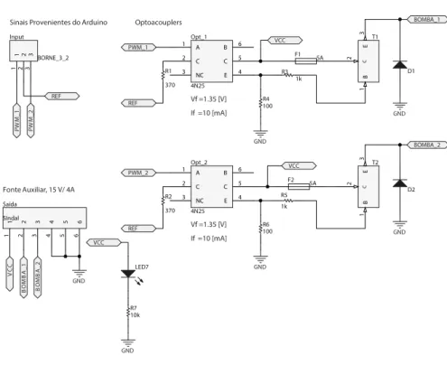
A 1 C 2 NC 3 E 4 C 5 B 6 Opt_1 4N25 A 1 C 2 NC 3 E 4 C 5 B 6 Opt_2 4N25 1 1 2 2 3 3 Input BORNE_3_2 P W M _ 1 P W M _ 2 REF 370 R1 PWM_1 REF PWM_2 370 R2 REF VCC B 1 C 2 E 3 T1 1k R3 100 R4 GND VCC D2 B 1 C 2 E 3 T2 1k R5 100 R6 GND BOMBA_1 BOMBA_2 Sinais Provenientes do Arduino
Fonte Auxiliar, 15 V/ 4A
Optoacouplers
Vf =1.35 [V] If =10 [mA]
Vf =1.35 [V] If =10 [mA]
1 1 2 2 3 3 4 4 5 5 6 6 Saída SIndal V C C B O M B A _ 1 B O M B A _ 2 GND D1 GND F1 5A F2 5A GND LED7 VCC 10k R7 GND
Source: The Author
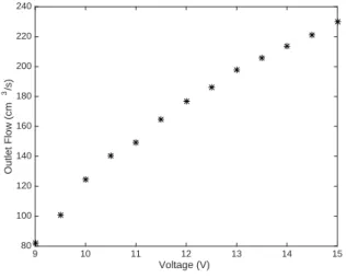
Chapter 2. Two-Tank System Modeling 29 defined by two times, the first beingTon, which is the amount of time in which the signal is in the upper level, while the second, To f f, is the amount of time in the lower level. The relation between Ton and the PWM period defines a percentage of which the average of the signal is directly dependent. For further details on PWM see (UMANAND, 2009). Figure 8 illustrates the curve voltage versus outlet flow of the pumps.
Figure 8 – Operation range of the pumps
9 10 11 12 13 14 15
Voltage (V)
80 100 120 140 160 180 200 220 240
Outlet Flow (cm
3/s)
Source: The Author
The Flow Measurement
The flow measurement is taken by a flow sensor model YF-S201, shown in Figure 9, whose principle is based on the hall effect. This sensor gives a square wave as output with
Figure 9 – Flow Sensor Model YF-S201
Source: The Author
frequency proportional to the flow rate passing by. A typical response of this sensor as well as the measurements taken from one of the sensors are given in Figure 10.
The Height Measurement
Chapter 2. Two-Tank System Modeling 30 Figure 10 – Output of the flow sensors
10 20 30 40 50 60 70 80 90 100 110
Frequency (Hz)
0 50 100 150 200 250
Flow rate (cm
3/s)
Typical Measured S1
Source: The Author
Figure 11 – Differential pressure sensor
Source: The Author
the fact that independently of the object’s shape the pressure is given by (HALLIDAY; RESNICK; WALKER, 2013):
∆P=ρgh (2.18)
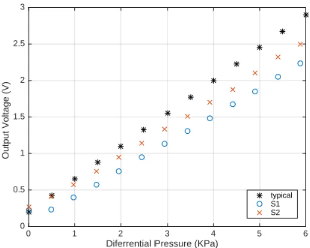
where∆Pis the differential pressure,ρ is the specific weight of the liquid,gis the gravitational acceleration andhis the liquid’s height. Ifg,ρ andPare known then the heighthis found from Eq. 2.18 accordingly. Both Earth’s gravitational acceleration and water’s specific weight are known, while the sensor gives the differential pressure. This makes possible the liquid’s height measurement in the tanks. The sensor gives a linear voltage output according to the pressure level. Figure 12 shows a typical pressure versus voltage curve of a MPX5010 and an actual curve of both sensors (Tanks 1 and 2). The real curve was obtained as the average of ten experiments. The calibration was done using a ruler to measure the real liquid height.
The Valve Opening Measurement
Chapter 2. Two-Tank System Modeling 31 Figure 12 – Curve voltage versus differential pressures
0 1 2 3 4 5 6
Diferrential Pressure (KPa)
0 0.5 1 1.5 2 2.5 3
Output Voltage (V)
typical S1 S2
Source: The Author
Every time that the valve changes its position the resistance of the potentiometer also changes. Thus, a voltage divider is used to measure the valve’s aperture. It is important to notice that this method can only map the percentage of the valve’s aperture when the minimal and maximum voltage are known. Figure 13 illustrates the real system.
Figure 13 – Valve’s aperture measurement
Source: The Author
2.6 The Experimental setup
As mentioned previously, in order to estimate the constantkfor each valve, it is neces-sary to perform dedicated experiments. In this section these experiments will be the focus of discussion.
Chapter 2. Two-Tank System Modeling 32 accomplished for both exit valves of each tank. For such experiment, a data setqj,hj
N j=1will
be collected, and based on it the value ofkcan be estimated .
Table 2 and 3 show, respectively, the data set collected from the experiment using the valves from Tank 1 and 2. Eachkfrom both valves were estimated using the Least Squares (LS) algorithm. See Sec. 3.4 for further details.
Table 2 – Data set from Tank 1’s valve
Flow (cm3/s) 216.2 202.6 192.1 186.8 176.3 165.8 157.4 149 141.7 133.3 Height (cm) 51.5 44.5 38.5 34.5 30 24.5 20 15 12.5 9.5
Source: The Author
Table 3 – Data set from Tank 2’s valve
Flow (cm3/s) 220.4 209.9 199.4 190 180.5 170 159.5 150.1 139.6 129.1
Height (cm) 55 48.5 43 37.5 32.5 28 22 17 12.5 9
Source: The Author
2.7 Summary of the Chapter
33
3 THE LINEAR PARAMETER-VARYING SYSTEM IDENTIFICATION
In this chapter are shown the methods used to identify models in the framework of Linear Parameter-Varying (LPV) systems. In order to understand the dynamic behavior and what an LPV system is, it will be first described the basic properties of LPV systems in section 3.1,i.e., its input-output relationship in association with the scheduling signal. In this context will be presented the model structures of LPV systems in section 3.2, such as input-output (IO) and state space(SS) representation. Following, methods to parametrically estimate these models are examined in sections 3.3-3.5. In sequence, it will be shown a non-parametric strategy to estimate LPV Models in an input-output setting in section 3.6. An extension of the previous method that delivers unbiased estimates regardless of the noise structure is given in section 3.7.
3.1 LPV Systems
The LPV system framework was originally introduced by Shamma (1988). The idea was to extend the gain-scheduling technique (ÅSTRÖM; WITTENMARK, 1994), which is a design approach that constructs nonlinear controllers considering a nonlinear plant as an array of linear plants in many operational conditions. In the LPV framework, the so-called scheduling variable p, usually an external signal, plays an important role, it represents a dynamic mapping between inputuand outputy. In this way, both have parameters that are p-dependent. As a matter of fact, LPV systems can describe both nonlinear behavior and time-varying phenomena, while keeping the attractive structure of a linear system. In fact, for a constant signal pan LPV system behaves exactly as an LTI system. Regarding the LTI system theory, an LPV system can be seen as a collection of LTI systems interpolated by a scheduling function (based on p).
The LPV systems can be represented as a convolution depending onuand p, which in discrete time is represented as (TÓTH, 2010):
y(k) =
∞
∑
i=0gi(p)q−iu(k), (3.1)
whereqdenotes the forward/backward time shift operator, i.e.q−iu(k) =u(k−i),u:Z→Rnu
is the discrete input,y:Z→Rny is the discrete output, and p:Z→Pis the scheduling variable
of the system with scheduling spaceP⊆Rnp. The coefficientsg
iin Eq. 3.1 are functions of the scheduling variable and they define the varying dynamical relation between uand y(TÓTH, 2010). Additionally, there are two types of dependence related to time on p: the static and dynamic dependence. The former is when the coefficientsgidepend only on instantaneous values of p, i.e.y(k) =g0(p(k))u(k) +g1(p(k))u(k−1)..., whereas the latter is defined by coefficients
that depend on time-shifted versions of p, i.e.y(k) =g0(p(k),p(k−1))u(k) +g1(p(k),p(k−
Chapter 3. The Linear Parameter-Varying System Identification 34 LPV system described by Eq. 3.1 is equivalent to an LTI system, where the coefficientsgiare constants. See (OPPENHEIM; WILLSKY; HAMID, 1996) for the definition of convolution in LTI systems. Figure 14 shows the relationship between aforementioned variables.
Figure 14 – LPV System
y(k)
u(k)
p(k)
LPV
Source: The Author
3.2 LPV Model Structures
There are two basic types for LPV model representation: the IO and SS structures. These are based on the well-established LTI framework, see (OPPENHEIM; WILLSKY; HAMID, 1996) for details. Again, the similarity between LPV and LTI systems are advantageous in terms of application. The equivalence between model structures IO and SS in the LPV framework is, in general, more complicated than the LTI counterpart, as in the LPV case usually involves dynamic dependence on the scheduling variable(TÓTH, 2010). In this thesis, it will be explored the LPV-IO representation. Although the SS structure allows the insertion of noise in the model, the IO setting allows a clear separation between process and noise structures. In this way, IO representation gives a better understanding of the model stochastic properties. Moreover, the IO representation is relatively easier to parametrize and doesn’t suffer from explosions of data (curse of dimensionality), contrary to the SS representation (VAN WINGERDEN; VERHAEGEN, 2009).
The LPV-IO Representation
This particular representation originates from the difference equation (discrete time) and is well-established in the LTI framework (OPPENHEIM; WILLSKY; HAMID, 1996). The LPV-IO representation describes the system input-output behavior by using polynomial equations in terms of the forward/backward time-shift operator. The model is generally described in a filter form:
y(k) =− na
∑
i=1ai(p)q−iy(k) + nb
∑
j=0bj(p)q−ju(k), (3.2)
where the coefficients{ai}ni=a1,
Chapter 3. The Linear Parameter-Varying System Identification 35 on p. The case wherena=0, meaning that there is no output dynamic involved is known as Finite Impulse Response (FIR) model.
Usually in real world applications, the model represented in Eq. 3.2 is just an abstraction of the deterministic behavior of the system and, in general, it can barely represent the system behavior. Therefore, a noise must be regarded in order to take into account uncertainties of the system. Typically, the noise added is white noise or a filtered version of it. Hence, the model in Eq. 3.2 is described as following:
y(k) =− na
∑
i=1ai(p)q−iy(k) +q−nk nb
∑
j=0bj(p)q−ju(k) +e(k), (3.3)
wheree(k)is a zero-mean white noise process andnkis the dead time. This model is the LPV version of the well-known ARX (Autoregressive with exogenous input) model from the LTI framework. Such model is part of a more general transfer function family. See (LJUNG, 1999) for further details on the LTI models.
The LPV-SS Representation
Similar to the LTI case, the LPV models have a state space representation, see (OPPEN-HEIM; WILLSKY; HAMID, 1996) for more details on LTI-SS structure. An LPV-SS model is generally described as:
qx=A(p)x+B(p)u,
y=C(p)x+D(p)u,
(3.4a) (3.4b)
wherex:Z→Rnx is the state-variable and A(p)∈Rnx×nx ,B(p)∈Rnx×nu,C(p)∈Rny×nx,
D(p)∈Rny×nuare matrix functions with static dependence on p. In the LPV framework, most
of the control synthesis assumes a state space representation as model.
3.3 LPV Identification Approaches
The first difference on the identification procedure of LPV systems is the necessity to measure a third signal entity, which is the scheduling variable. Usually for identification of LTI systems, a data set in the form{uk,yk}Nk=1 must be collected, whereas in the LPV framework
this data set must include the scheduling variable. Hence, the data set must be in the form
DN={uk,yk,pk}Nk=1. (3.5)
Chapter 3. The Linear Parameter-Varying System Identification 36 can be achieved by maintaining a constant pwhile collecting the data. Recall that for a constant scheduling p(k) =p¯for anykthe LPV model is equivalent to an LTI model. Subsequently, the LPV system is obtained by an interpolation method, such as polynomial, radial basis functions, sigmoidal (TÓTH, 2010). When it comes to the global approach, a unique global structure assumption in the model within the scheduling space is considered, conversely of the local approach. However, the estimation problem using a local approach can be solved similar to the global approach, by considering only one data set ranging many sub-data sets in many working points. In (NOGUEIRA, 2012) was shown a local estimation approach using a global structure. One main drawback of this approach is the explosion of data (curse of dimensionality) as many working points are added. Such issue is unlikely to happen within the scope of a global approach, because of the global nature of the data collection.
In this thesis, it will be explored the methods within the scope of the global approach under the LPV-IO setting.
3.4 The Regression Approach
The regression approach is based on considering the one-step ahead predictor of the system model in regression form. This method lies on the prediction error method (PEM) (LJUNG, 1999), which includes the maximum likelihood method, as well. In order to extend the PEM for LPV systems, it is necessary to define the concept of LPV system description. Then, it is possible to obtain a general one-step-ahead predictor to formulate the identification under the mean-square error framework (MOHAMMADPOUR; SCHERER, 2012).
General LPV System Description
The general LPV system description can be extended from the LTI framework as a process filter with additive disturbance as:
y(k) =G(q,p)u(k) +v(k), (3.6)
whereG(q,p)is ap−dependent filter defined similarly as in Eq. 3.1. In (TÓTH, 2010) it was shown that this filter can be equivalently defined as a convolution betweenuandp. This definition is the LPV form of the impulse response (IR) in the LTI framework, where eachgi(p)is the LPV equivalent of the impulse response coefficients. It is assumed thatvis a quasi-stationary noise process with a bounded power spectral densityΦv(ω), and can be described by the following relationship:
v(k) =H(q,p)e(k), (3.7)
Chapter 3. The Linear Parameter-Varying System Identification 37 Figure 15 – Signal flow of the general LPV system descriptor
u(k)
G(q, p)
p(k)
++
y(k)
H(q,p)
e(k)
Source: The Author
General Assumptions Under LPV Identification Framework
A first assumption of the LPV framework stands the fact that the scheduling variable must be a measurable entity. Another common assumption in literature involving the scheduling variable is that measurements of pare noise free, see (BAMIEH; GIARRÉ, 2002; DANKERS et al., 2011; LOPES DOS SANTOS; RAMOS; MARTINS DE CARVALHO, 2007; LOPES DOS SANTOS et al., 2013; LAURAIN et al., 2011c; LAURAIN et al., 2012; LAURAIN et al., 2010a; TÓTH et al., 2011; LAURAIN et al., 2010b), exceptions are (BUTCHER; KARIMI; LONGCHAMP, 2008; PIGA et al., 2015; ABBASI et al., 2014). The main reason for the assumption of the noise free observations of the scheduling variable lies on issues regarding the conditional expectation of v(k) when the true observation of p is not available, as each coefficient of the filter defined in Eq. 3.7 can be a nonlinear function with dynamic dependence on p(MOHAMMADPOUR; SCHERER, 2012). This is a quite non-realistic scenario since, generally, observations of the scheduling variable are subject to uncertainties, such as, noise measurements due to sensors and experimental conditions.
In this thesis, it will be considered the case where truep, which is the noise-free version of the scheduling variable, is available.
The One-Step Ahead Prediction ofv
In order to formulate the estimation of parametric LPV models in the PE setting, it is necessary to characterize the one-step ahead predictor ofy(MOHAMMADPOUR; SCHERER, 2012). Consequently, a one-step ahead prediction of the noise process is necessary to formu-late the prediction error. To do so, the filter H(q,p)must be stable and it must have a stable inverse, which means that, there exists a monic convergent filter denoted asH†(q,p)such that
H†(q,p)H(q,p)=1 (TÓTH, 2010). This implies that Eq. 3.7 can be rewritten as:
Chapter 3. The Linear Parameter-Varying System Identification 38 and similarly to the LTI case, it can be shown that the one-step ahead predictor of v(k)is the following (TÓTH, 2010):
v(k|k−1) =1−H†(q,p)v(k). (3.9)
The One-Step Ahead Prediction ofy
To address the problem of estimation parametric LPV models minimizing the prediction error, which is the difference between the actual output and the predicted model output, it is necessary to define the one-step ahead predictor of the model outputy.
As an extension of the LTI case (LJUNG, 1999), it was shown that under theptrue case with information aboutyk−1={y(τ)}τ≤k−1,uk={u(τ)}τ≤k, and pk={p(τ)}τ≤k, the one-step ahead output predictor is (TÓTH, 2010):
y(k|k−1) =
H†(q,p)G(q,p)u(k) +1−H†(q,p)y(k). (3.10)
Parametrization of LPV Models
In order to write the LPV-IO model in the regression, the scheduling variable dependen-cies must be well-defined. The main requirement is that the model must be linear in parameters. To parametrize the model it will be considered that each parameter of the filterA(p)andB(p) can be decomposed in terms of a priori selected basis setψi j:P→R. Then fori=1, ...naeach element ofA(p)in Eq. 3.2 can be defined as:
ai(p(k)) =θi0+θi1ψi1(p(k)) +···+θilψisi(p(k)), (3.11)
whereθi j∈Rare the unknown parameters to be identified. Similarly, each element ofB(p)in Eq. 3.2 can be defined fori=0, ...nbas:
bi(p(k)) =θi0+θi1ψi1(p(k)) +···+θilψisi(p(k)). (3.12)
It is possible to select a functionφ(·)that generalizes the dependency onp(k)for each parameter of the LPV-IO model. In this way, the process part is fully characterized by {φi(·)}in=a+1nb+1. Therefore, the LPV model in a regression form must be linearly parametrized as follows:
φi(·) =θi0+ si
∑
j=1θi jψi j(·), (3.13)
once this parametrization is chosen, it becomes possible to pose the estimation problem in a regression form. As pointed in (BAMIEH; GIARRÉ, 2002) there are many possibilities for the choice of the basis functions, such as, monomials, periodic functions like sine and cosine, and sigmoidal. It is a common assumption in literature that this parameter dependency is of polynomial form, see (BAMIEH; GIARRÉ, 2002; BUTCHER; KARIMI; LONGCHAMP, 2008; LAURAIN et al., 2010b). This corresponds to the following parametrization:
Chapter 3. The Linear Parameter-Varying System Identification 39
MIMO LPV-IO Models
In this thesis, it will be dealt mainly with multiple inputs multiple outputs (MIMO) systems. For this reason, a formal characterization of these models in an IO setting is necessary. The extension to MIMO LPV-IO is accomplished similarly for the LTI case (LJUNG, 1999). The MIMO LTI-ARX model can be described as in Eq. 3.3 by analogy (LJUNG, 1999):
y(k) =− na
∑
i=1AAAiq−iy(k) + nb
∑
j=0B B
Bjq−nk−ju(k) +e(k), (3.15)
withy∈Rny the vector output, u∈Rnu the vector input, and the coefficient matrices A
i, Bj defined as:
y(k) =y1(k)···yny(k) T
, u(k) = [u1(k)···unu(k)]
T
, (3.16)
A AAi=
ai,1,1 ··· ai,1,ny
... ... ... ai,ny,1 ··· ai,ny,ny
, BBBj=
bi,1,1 ··· bi,1,nu
... ... ... bi,ny,1 ··· bi,ny,nu
, (3.17)
wheree(k) =e1(k)···eny(k)
T is a white noise stochastic vector. However, this model assumes that each output channel has influence over each other, leading to dynamics of each output influencing each other. A common approach in dealing with MIMO systems is to assume that there is no influence in dynamics from other outputs. In this way, the matrix AAAi in Eq. 3.17 assumes the following form:
A A Ai=
ai,1 ··· 0 ... ... ... 0 ··· ai,ny
, (3.18)
Using this parametrization, identification of a MIMO LTI system can be performed separately for each output via the estimation of multiple input single output (MISO) systems (LJUNG, 1999). In fact, it is preferable to cope with the estimation ofnyMISO systems than a MIMO system, mainly to avoid overparametrization due to the presence of zeros on the regressors. To extend this model to the LPV-ARX case it is just necessary to allow the coefficients in matrices to depend on p, by using the LPV matricesAAAi(p(k))andBBBj(p(k)):
A A
Ai(p(k)) =
ai,1,1(p(k)) ··· 0
... ... ...
0 ··· ai,ny,ny(p(k))
,BBBj(p(k)) =
bi,1,1(p(k)) ··· bi,1,nu(p(k))
... ... ...
bi,ny,1(p(k)) ··· bi,ny,nu(p(k))
,
(3.19)
with the following equation defining the MISO LPV-ARX Model:
y(k) = na
∑
i=1A
AAi(p(k))q−iy(k) + nb
∑
j=0B
Chapter 3. The Linear Parameter-Varying System Identification 40 Wherey(k)is a scalar corresponding to one specific output of the MIMO system,u(k)is defined in Eq.3.16 andAAAi,BBBj are defined as in Eq.3.19. In the case of the MIMO LPV-ARX system, the setφi,j
ny,nt
i=1;j=1fully characterizes the dependence on the scheduling variable, with each basis
function as in Eq. 3.13:
φi,j(·) =θi,j,0+ si j
∑
k=1θi,j,kψi,j,k(·), (3.21)
withnt=na+nu(nb+1), and eachφi,jis a real function with static dependence on p(k).
Estimation via the LS Criterion
It is possible to write the LPV-IO model as a linear regression form using Eqs. 3.3 and 3.13. Firstly, it is necessary to write the LPV model in a linear regression form as:
y(k) =ϕT(k)θ+e(k), (3.22)
wherey is the output, ϕ is the regression vector,θ is the parameter of the model and eis a gaussian white noise process. For the LPV-ARX model defined in Eq. 3.3, this transformation is straightforward. However, in order to write this model in regression form, it is first required to choose appropriate basis functions that properly parametrize the model in pas in Eq. 3.13. Choosing a linear in parameters basis function leads to coefficients of filterAandBin the form of Eqs. 3.11-3.12. Then, the parameter and regression vectors in Eq. 3.22 for the LPV-ARX model will be the following:
θT =hθ10 ···θ1s1θ20···θ2s2···θnasnaθna+10···θna+1sna+1···θngsng i
ϕT(k) =h
−y(k−1)−y(k−1)ψi1(p(k))··· −y(k−na)ψnasna(p(k))···
u(k−nk) u(k−nk)ψna+11(p(k))··· u(k−nk−nb+1)ψngsng(p(k)) i
(3.23a)
(3.23b)
whereng=na+nb+1. The MISO LPV-ARX can be parametrized in a similar fashion. It is only necessary to add the additional inputs and their respective parameters in the regression equation. The only requirement is that the whole model must be linear in parameters. Then, the regressors and the parameter vectors of the MISO LPV-ARX can be defined as follows:
θT =θ10 ···θ1s1θ20···θ2s2···θnasnaθna+10···θna+1sna+1···θntsnt
ϕT(k) =h−y(k−1)−y(k−1)ψi1(p(k))··· −y(k−na)ψnasna(p(k))···
u1(k−nk) u1(k−nk)ψ1,na+1,1(p(k))··· u1(k−nk−nb+1)ψ1,ng,sng(p(k))···
unu(k−nk) unu(k−nk)ψnu,na+1,1(p(k))··· unu(k−nk−nb+1)ψnu,ng,sng(p(k)) i
(3.24a)
(3.24b)
with the first index of θi,j,k, and ψi,j,k not used because there is only one output for MISO systems. The Least Squares criteria is based on the minimization of the mean square error, which is summarized in the following cost function:
VN = 1 N
N
∑
i=1Chapter 3. The Linear Parameter-Varying System Identification 41 with the LS estimates as a minimizer defined as follows:
θLS=argminVN, (3.26)
it is well-known that for the linear regression case the minimum of Eq. 3.25 can be found as follows, by definingYYY = [y(1)y(2)···Y(N)]T andΦΦΦ= [ϕ(1)ϕ(2)···ϕ(N)]T (LJUNG, 1999):
θLS=ΦΦΦ†YYY, (3.27)
whereΦΦΦ†= N1ΦΦΦTΦΦΦ−1 1NΦΦΦT is the regularized version of the Penroe-Monrose pseudoinverse (LJUNG, 1999; MOHAMMADPOUR; SCHERER, 2012). This solution is identical to the LTI case (LJUNG, 1999), which is possible because an LPV system can be viewed as a multiple input single output (MISO) LTI model with virtual inputs as pointed in (MOHAMMADPOUR; SCHERER, 2012; LAURAIN et al., 2010a; LAURAIN et al., 2010b). However, it is well-known that the minimizer in Eq. 3.27 leads to an unbiased estimate if the noiseein Eq. 3.22 is white, which is only true for the ARX model structure (LJUNG, 1999; MOHAMMADPOUR; SCHERER, 2012).
Recursive Versions of the LS Algorithm
The adopted LS approach herein is based on the classical approach, which considers the regression vector stacked as column. As the LPV-ARX model can be viewed as an LTI MISO system, other type of parametrizations arise. In (BAMIEH; GIARRÉ, 2002) it was shown that the least mean squares (LMS) and recursive least squares (RLS) algorithms can be extended to the LPV case. A parametrization similar to the MISO LTI models was chosen (LJUNG, 1999), where the regression and parameter vectors in Eqs. 3.23a, 3.23b are matrices, instead of vectors.
The parametrization is then performed in the following way. Define the parameter matrix ΘΘΘ∈Rng×np, withn
pbeing the number of basis functions, as:
Θ ΘΘ:=
a11 ··· an1p a12 ··· an2p ... ... ... a1na ··· annap
b10 ··· bn0p ... ... ... b1nb ··· bnnbp
. (3.28)