Engineering ISSN: 1809-4430 (on-line)
_________________________
1 Key Laboratory of High Efficiency Clean Machinery Manufacturing, Ministry of Education, College of Mechanical Engineering,
Shandong University/ Jinan, China.
3 SAIC Commercial Vehicle Technology Center/ shanghai, China.
MEASUREMENT AND ANALYSIS OF A FIELD AREA BASED ON AN ADAPTIVE KALMAN FILTER
Doi:http://dx.doi.org/10.1590/1809-4430-Eng.Agric.v37n5p867-876/2017
SUSU FANG1, ZENGCAI WANG2*, WENJUN ZHONG3
2*Corresponding author.Key Laboratory of High Efficiency Clean Machinery Manufacturing, Ministry of Education, College of Mechanical Engineering, Shandong University/Jinan, China. E-mail: [email protected]
ABSTRACT: This paper proposed the use of an adaptive Kalman filter (AFK) to improve Global Positioning System (GPS) positioning accuracy to measure a tractor operational area. First, we used MATLAB to identify the operation trajectory. Then, we used different colors to show the area of operation. Finally, we used an image-processing method to calculate the effective operational area, actual operational area, and repeat and omission rates. We used these rates to evaluate the tractor efficiency. The experiment indicated that the Kalman filter improved the accuracy of GPS single-point positioning. To test the GPS area-measurement precision, field area measurements were taken. We used GPS to measure standard figures and some irregular figures. The results indicate that the area measurement relative error was 2.09%. The measurement accuracy increased with the increasing measurement area. The field test results indicated that the most efficient farming method was alternative tillage and the second most efficient was spindle tillage. The omission rate under back tillage was highest and its operational efficiency was lowest.
KEY WORDS: tractor, Kalman filter, Global Positioning System (GPS), operational area.
INTRODUCTION
Area measurement has been extensively used in precision agriculture, precision forestry, and land surveying (Cavallo et al., 2014; Mitri, 2014; Simikić et al., 2014). The traditional measurement of field areas has been through manual measurement. The efficiency of this approach is low and the accuracy is poor. With the rapid development of science and technology, GPS measurement has become a convenient approach and is widely used in agricultural machinery navigation, positioning and operational area measurements (Langer et al., 2015; Shahgholi & Abuali, 2015). In the measurement of a field area, GPS has become an important measurement tool that has completely changed the traditional approach to operations, reduced labor, and improved production efficiency (Mehta & Tewari, 2015; Lee et al., 2016).
The rapid development of modern agriculture in China has generated advanced requirements for agricultural machinery. During farm work, as a result of manual tractor operation, the adjacent trajectory between two operational lines can produce repeated areas and missing areas. It is necessary to solve the issue of how to accurately measure the area of operation. This paper proposed using an adaptive Kalman filter (AKF) to improve the GPS positioning accuracy to accurately measure the tractor operational area. The AKF algorithm is more suitable in the case of unknown noisy statistics or in the case of an inaccuracy.
MATERIAL AND METHODS
( ) ( 1) ( )
X k FX k Gw k (1) where,
F represents the state transition matrix;
( )
X k represents the state vector at sample time k;
G represents the process noise gain matrix;
( )
w k represents the process noise and takes into account the perturbations in the system, and
Q represents the process noise covariance matrix.
The measurement model provides the relationship between the system states and the physical quantities measured by the sensor (Kayacan et al., 2015). This relationship can be represented in a generalized formulation in discrete time as follows:
( ) ( ) ( )
z k HX k v k (2)
where,
( )
z k represents the measurement vector obtained from the sensor;
Hrepresents the observation matrix;
( )
v k represents the measurement noise, and
Rrepresents the positive definite covariance matrix of the measurement noise.
The position and velocity of the static point-positioning model of the receiver was the state vector, and the state vector was set asX[x x x y y y z z z]T.
where,
x represents the latitude;
y represents the longitude and z represents height;
x represents the latitude velocity;
y represents the longitude velocity and z represents the height velocity, and
x,y andz are the acceleration in three ways.
Using the constant velocity model, the parameters were as follows: State transition
matrix 0 0 0 0 0 0 Φ F Φ Φ , 2
1 / 2
0 1
0 0 1
T T T
Φ . The process noise gain matrix
0 0 0 0 0 0 ς G ς ς , 3 2 / 6 / 2 T T T
ς . The
observation matrix
1 0 0 01 0 0 0 1
H . The positive definite gain matrix of the measurement
noise 2 2 2 0 0 0 0 0 0 x y z σ σ σ
R , 2 2.4 104
x
σ
, σ2y 1.5 104
, 2 0
z
σ , where T represents the sampling time
(Du & Ren, 2008). The mean value before filtering was chosen as the initial value of the Kalman
filter (Sun et al., 2013): T
0[ 0 0x y 0 0z 0 0]
X . The discrete sampling time was T1s.
divergence of the system was degraded. The AKF algorithm for system noise estimation was mainly based on the application of covariance matching technology and a new interest sequence of the Kalman filtering algorithm (Sun et al., 2013).
The implementation steps of the AKF algorithm was as follows:
(1) Initialization: Qˆ0Q0,Rˆ0R0;
(2) Time update (effect dynamics);
| 1 1
2
| 1 | 1
0
2 | 1 | 1
| 1 0
| 1 | 1
| 1 | 1
2
| 1 | 1
0 ˆ ˆ ˆ ˆ ˆ i i k k k
n
m i k k i k k
i
i
n k k k k c
k k i T
i i
k k k k k
i i k k k k
n m i k k i k k
i
X H X
X W X
X X
P W
X X
Q
z H X
z W z
(3)(3) Measurement update (effect of measurement);
2 | 1 | 1
, 0
| 1 | 1
2 | 1 | 1
, 0
| 1 | 1
1
, ,
| 1 | 1
, | 1 ,
ˆ
ˆ ˆ
ˆ
ˆ
ˆ ˆ ˆ
i
n k k k k c
yy k i i T k i
k k k k i
n k k k k c
xy k i T i
i
k k k k xy k yy k
k k k k k k T xx k k k yy k
z z
P W R
z z
X X
P W
z z
K P P
X X K z z
P P KP K
(4)(4) Update system noise statistics;
1 | 1 0 1 ˆ N T T
k k j k j k k k k j
R ε ε H P H
N
(5)
1 1
0 0
| 1 ,
1
ˆ N N
T T T
k k k k j k j k j k j
j j
T k k k xx k k
H Q H ε ε η η
N
H P P H
(6)coordinates (Zhang et al., 2009), including the geodetic coordinates
B L,
, were solved for theGauss plane Cartesian coordinates
x y, .The Gaussian projection exhibited length deformation, but this was unavoidable. However, certain measures must be taken to limit it, and the method to limit the length deformation was to create zoning. So-called zoning was the projection region within a narrow range of a central meridian for the symmetrical axis. Generally, the zones were divided into 3 degrees and 6 degrees, 3 degrees of zoning to earth in 45 units, 6 degrees from earth were divided into 23 units; therefore, we tried to transform the longitude and latitude into zoning in the axis of symmetry on both sides. Only in this way could we reduce the projection deformation. In this paper, the measurement data had approximately 117 degrees of longitude, and the thirty-ninth zoning with 3 degrees of projection was selected.
GPS was installed on the tractor, which collected fixed position coordinates at certain time-steps. The tractor produced a large number of tracks when operating on the field. By collecting the trace, it generated a working path line; then, we were able to obtain the area of operation. The point trace was described as D
x y1, 1 , x y2, 2, ,x yn, n
. The working area of the tractor isdescribed as the effective operating area and the actual operating area.
(1) Effective operating area:
The effective operating area was the area of the polygon that was surrounded by the farmland
boundary (Luo & Zhong, 2005). The coordinates of the polygon was
1, 1 , 2, 2 , , i, i , i1, i1
D x y x y x y x y , where
1
1, 1 i1, i
x y x y .
The formula was as follows:
1
1
1
1 2
n
i i i i i
S x x y y
ea
(7)
The perimeter of the polygon was as follows:
2
21 1
1
n
i i i i i
L x x y y
(8)(2) Actual operating area:
To calculate the actual operating area, the actual working trajectory of the tractor in the field needed to be recognized. The tractor working width was known as M(m). The length of the trajectory was considered to calculate the area of actual operation:
2
2ac 1 1
1
S = M
n
i i i i i
x x y y
(9)The operation efficiency of the tractor was judged based on the repeat to omission ratio. The repeat rates and omission rates were small; the operation efficiency was high, and vice versa. The repeat rate was equal to the repeat area to the effective area, and the rate of omission was equal to the ratio of the omission area to the effective area.
acquisition frequency of 1 s. Because the main purpose of this paper was to calculate the field area, we only considered the longitude and latitude ( , )B L direction in the calculation and translated the
collected data through the Gaussian into plane coordinates. We used the Kalman filter algorithm to address the data; then, we obtained the results.
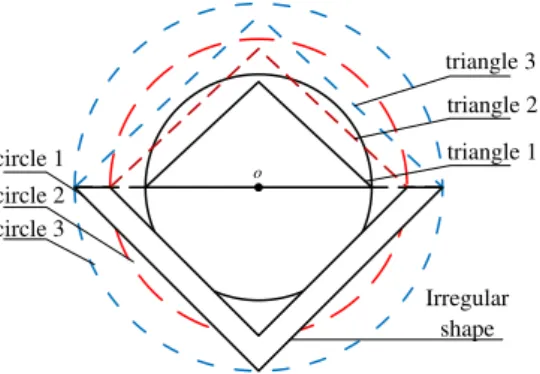
To verify the accuracy of the GPS area measurement, the measurement results of the GPS single point positioning method was verified using measurements of the circular, triangular and irregular patterns. This paper chose three circles with radii of 3 m, 4 m, and 5 m as well as three isosceles triangles and irregular graphics for inclusion in a measurement figure, as shown in Fig. 1.
o
Irregular shape
triangle 3
triangle 2
triangle 1 circle 1
circle 2 circle 3
FIGURE 1. Graph of ground measurement.
After verifying the accuracy, experimenters used handheld GPS while walking along the experimental field boundary to measure the experimental field area. Furthermore, we used tape to measure the length and width of the field to directly calculate the area of the plots. A comparison of the two ways to measure the size of the area could evaluate the method of GPS measurement area with more accuracy. The blocks are shown in Fig. 2.
FIGURE 2. The block boundary of GPS measurement.
FIGURE 3. Experiment block segments.
based on the different methods of tillage, including back tillage, spindle tillage, and alternative tillage. The Experimental procedure was as follows: (1) a tape was used to measure the length and width of the three experimental blocks, which were measured three times; (2) an artificial hand G HiPer II receiver was used while walking three times around the experimental field boundary to identify the field boundary, we took each field measurement twice; (3) a rotary tiller 1GQN200 and
G HiPer II receiver were installed on the WD854 tractor and the tractor’s working width was 2 m. A
rotary tillage experimental field was established using the three selected tillage methods, and a computer obtained real-time data and saved the GPS data to a computer laptop. The GPS data acquisition involved the serial communication principle. LabVIEW software was used to read the GPS serial data, which we saved to Excel; this was convenient for subsequent data processing. The effective area and the actual operating area of the experimental plot were calculated in computer programming software, and we calculated the repeat and omission rates of different blocks.
RESULTS AND DISCUSSION
(1) The verification results ofsingle point positioning accuracy
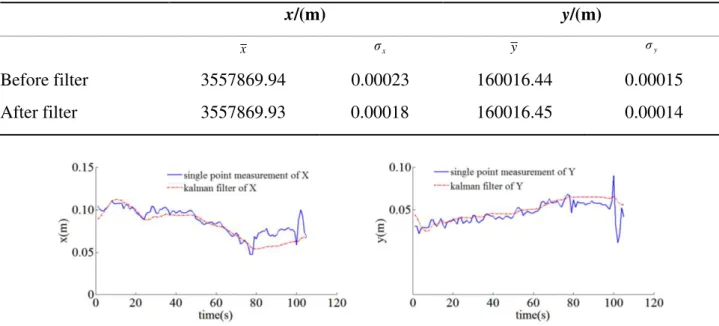
The Kalman filter algorithm was used to filter the x and y values; the filtered results are shown in Table 1.
TABLE 1. Mean and mean square error of the x and y directions before and after filtering.
x/(m) y/(m)
x σx y σy
Before filter 3557869.94 0.00023 160016.44 0.00015
After filter 3557869.93 0.00018 160016.45 0.00014
FIGURE 4. Change curves of the x and y directions before and after filtering.
To clearly show the range of the numerical values, the longitudinal coordinate data in Fig. 4were part of the integer portion of the data. From Figure 3, we can see that the wave of the numerical fluctuation in front of the filter, x and y were relatively large, and the numerical changes of y and x after filtering were mild. The mean values of the coordinates of the filter were small, and the changes of the mean values were small. After filtering, the positioning accuracy was improved, such that the accuracy of the area was improved.
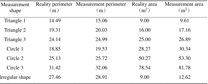
(2)The verification results of the accuracy of the GPS area measurement
TABLE 2. Perimeter and area of the measurement shape.
Measurement shape
Reality perimeter
(m)
Measurement perimeter
(m)
Reality area
(m2)
Measurement area
(m2)
Triangle 1 14.49 15.06 9.00 9.61
Triangle 2 19.31 20.03 16.00 17.16
Triangle 3 24.14 24.99 25.00 26.89
Circle 1 18.85 19.53 28.27 30.34
Circle 2 25.13 25.72 50.27 53.30
Circle 3 31.42 32.06 78.54 81.78
Irregular shape 27.46 28.91 9.00 12.62
(3) Analysis of the field test results
The total area of the experimental field was measured with GPS, and the total area was 4055.05 m2; the relative error was 2.09%, as shown in Table 3.
TABLE 3. Area and relative error of the experiment blocks.
Test No. GPS method (m2) Tape method (m2) Relative error
First test 3931.42 4156.25
2.09%
Second test 4095.30 4127.34
Third test 4138.44 4141.49
Average value (m2) 4055.06 4141.70
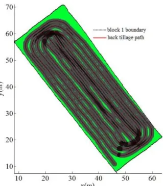
The results from the three blocks with different methods are described below. Block 1 used the back tillage method, as shown in Fig. 5. The effective area of the plot used a GPS measurement of 1440.27 m2. We obtained the operation trajectory of the back tillage. At this time this part of the
track was not working. The actual operational area of the block was 1323.58 m2, the repeat rate was
6.19%, and the omission rate was 14.29%. A large area was missing tillage, which mainly occurred in the fields at both ends, and the rotary tillage fields were increased in this section. The efficiency of back tillage was low, and the operation time was long.
Block 2 used the spindle tillage method, as shown in Fig. 6. It also used the GPS-measured effective area of 1346.19 m2. In the calculation of the actual operational area, the field U-turns
produced in the track area were subtracted. The spindle tillage method had an invalid operation (head, U-turn), and this increased the operational time. The actual operational area of the block was 1276.49 m2, the repeat rate was 5.54%, and the omission rate was 10.72%. The spindle tillage
omission area was relatively large and appeared in the fields at both ends.
The third tillage method block is shown in Fig. 7. The effective operational area was 1335.67 m2. The method of tilling arable land changed when the rotary was lifted, and there was no
operation. An alternative tillage method reduced the switching frequency and reduced the burden of agricultural labor, but increased the agricultural labor needed to predict the trajectory of cultivated land. When the block area was large, it reduced the repeat rate. The calculation of the actual work area subtracted the terrain boundary outside of the headland turning area. The actual operation area
was 1402.26 m2, the repeat rate was 6.82% and the omission rate was 1.81%. Based on the repeat
FIGURE 5. Back tillage. Green areas indicate the omissions, dark grey areas show the repeat areas, grey areas represent normal tillage; the same is true below.
FIGURE 7. Alternative tillage.
TABLE 4. Parameters of the experiment blocks.
Block name Effective area (m2) Working area (m2) Repeat rate (%) Omission rate (%)
Block 1 1440.27 1323.58 6.19 14.29
Block 2 1346.19 1276.49 5.54 10.72
Block 3 1335.67 1402.26 6.82 1.81
(4) Test results discussion
The calculations of the repeat and omission rates were related to the skill of the tractor driver. At present, most Chinese farmland still relies on manual agricultural operations (Xia, 2013). Through this study, we evaluated the efficiency of drivers, regulated the driver’s approach and improved the driver's skills; ultimately, this could improve the production efficiency. If this study was applied to an autopilot, we could find the most efficient way to farm.
The GPS positioning data were random, so the accuracy of each test may be different. The positioning data of the receiver was disturbed by many factors and exhibited obvious randomness. The measurement accuracy of each test was also different. In the experiment, the position of the receiver was used, and the GPS and Galilean satellites were used to locate the position; furthermore, the positioning accuracy was higher than that of the single system (Hu et al., 2014). In the experiment, we carried out three repeated static positioning data acquisitions on the same point; then, we processed the data and both of the three data results verified the conclusion.
In a single point positioning experiment, relative positioning was often obtained, and when the satellite was unevenly distributed, Cycle Slips occurred and accurate measurement accuracy could be not obtained (Liu & Yang, 2012). In the field experiment, the terrain was relatively open, there was no large obstruction to block the satellite signal, and the real-time monitoring of the number of satellites that participated in the test were basically more than 11 (GPS satellite and Galileo satellite) and ensured the accuracy of the measurement.
CONCLUSIONS
(1) To accurately measure the operational area of the tractor, an adaptive Kalman filter was
used to improve the GPS positioning accuracy. After application of the Kalman filter, the x and y
(2) The results of the field measurement experiment indicated that the highest efficiency tillage method was the alternative tillage method. The requirements of the alternative tillage method were high, and agricultural laborers needed to clear the land route. The omission rate under back tillage and spindle tillage was large, and those methods have a long operational time and low work efficiency, as shown in Tables 3 and 4.
(3) The method of image processing was used to calculate the repeat and omission areas. We used different colors to display the area of common tillage, repeat area, and omission area, and the location of the concrete gravity leakage could be seen intuitively. The operating efficiency could be used to guide actual agricultural production and to choose an operational mode with a higher efficiency.
REFERENCES
Cavallo E, Ferrari E, Bollani L, Coccia M (2014) Attitudes and behaviour of adopters of technological innovations in agricultural tractors: A case study in Italian agricultural system. Agricultural Systems 130:44-54.
Du X, Ren Z (2008) Precision analyze based Kalman filter for GPS static point positioning[J]. GNSS world of China 5:47-51.
Hu G, Gao S, Zhao Y (2014) Novel adaptive UKF and its application in integrated navigation[J]. Journal of Chinese Inertial Technology 22:357-367.
Kayacan E, Ramon H, Saeys W (2015) Towards agrobots: Identification of the yaw dynamics and trajectory tracking of an autonomous tractor[J]. Computers and Electronics in Agriculture
115:78-87.
Langer TH, Ebbesen MK, Kordestani A (2015) Experimental analysis of occupational whole-body vibration exposure of agricultural tractor with large square baler[J]. International Journal of
Industrial Ergonomics 47:79-83.
Lee JW, Kim JS, Kim KU (2016) Computer simulations to maximise fuel efficiency and work performance of agricultural tractors in rotovating and ploughing operations. Biosystems Engineering 142:1-11.
Liu DR, Yang D (2012) A method of inhibiting multi path signals in the GNSS code tracking loop[J]. GNSS world of China 37:9-16.
Luo ZQ, Zhong EJ (2005) Derivation of Formula for Any Polygonal Area and Its Applications[J]. College Mathematics 21:123-125.
Mehta CR, Tewari VK (2015) Biomechanical model to predict loads on lumbar vertebra of a tractor operator. International Journal of Industrial Ergonomics 47:104-116.
Mitri FG (2014) Single Bessel tractor-beam tweezers. Wave Motion 51(6):986-993.
Shahgholi G, Abuali M (2015) Measuring soil compaction and soil behavior under the tractor tire using strain transducer. Journal of Terramechanics 59:19-25.
Simikić M,Dedović N, Savin L, Tomić M,Ponjičan O (2014) Power delivery efficiency of a wheeled tractor at oblique drawbar force[J]. Soil and Tillage Research 141:32-43.
Sun G, Wang CM, Zhang AJ (2013) Comparison of filtering algorithms for GPS static point Positioning[J]. Journal of Nanjing University of Science and Technology(Natural Science) 35:80-85.
Xia ZQ (2013) Current Situation and Future of Agricultural Machinery Development in China[J]. Beijing Agriculture 24:186-187.