doi: 10.1590/0101-7438.2016.036.02.0279
PACKING CIRCLES WITHIN CIRCULAR CONTAINERS:
A NEW HEURISTIC ALGORITHM FOR THE BALANCE CONSTRAINTS CASE
Washington Alves de Oliveira
1*, Luiz Leduino de Salles Neto
2,
Antonio Carlos Moretti
1and Ednei Felix Reis
3Received February 20, 2015 / Accepted May 12, 2016
ABSTRACT.In this work we propose a heuristic algorithm for the layout optimization for disks installed in a rotating circular container. This is a unequal circle packing problem with additional balance constraints. It proved to be an NP-hard problem, which justifies heuristics methods for its resolution in larger instances. The main feature of our heuristic is based on the selection of the next circle to be placed inside the container according to the position of the system’s center of mass. Our approach has been tested on a series of instances up to 55 circles and compared with the literature. Computational results show good performance in terms of solution quality and computational time for the proposed algorithm.
Keywords: packing problem, layout optimization problem, nonidentical circles, heuristic algorithm.
1 INTRODUCTION
We study how to install unequal disks in a rotating circular container, which is an adaptation of the model for the two-dimensional (2D) unequal circle packing problem with balance behavioral constraints. This problem arises in some engineering applications: development of satellites and rockets, multiple spindle box, rotating structure and so on. The low cost and high performance of the equipment require the best internal configuration among different geometric devices.
This problem is known aslayout optimization problem(LOP), and consists in placing a set of circles in a circular container of minimum envelopment radius without overlap and with mini-mum imbalance. Each circle is characterized by its radius and mass. There, the original three-dimensional (3D) case (the equipment must rotate around its own axis) is simplified: different
*Corresponding author.
1Faculdade de Ciˆencias Aplicadas, Universidade Estadual de Campinas, 13484-350 Limeira, SP, Brasil. E-mails: [email protected]; [email protected]
2Instituto de Ciˆencia e Tecnologia, Universidade Federal de S˜ao Paulo, 12247-014 S˜ao Jos´e dos Campos, SP, Brasil. E-mail: [email protected]
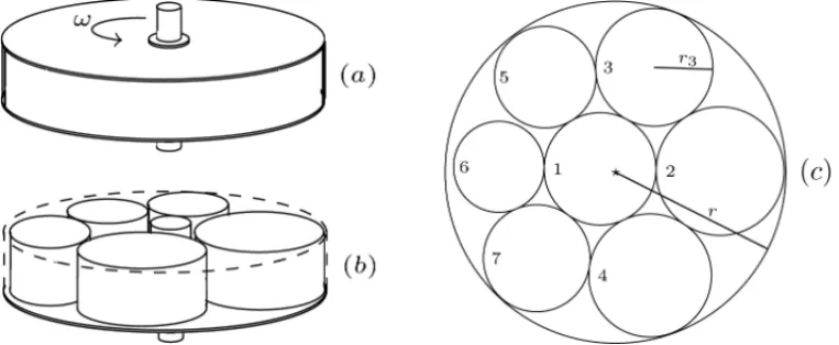
two-dimensional circles (see, Figure 1(c)) represent three-dimensional cylindrical objects to be placed inside the circular container.
Figure 1 illustrates the physical problem. Figure 1(a) shows a rotating cylindrical container. The symbolωand the arrow illustrate the rotation around the axis of the equipment,ωis the angular velocity. In another viewpoint, Figure 1(b) shows the interior of the equipment where distinct circular devices need to be placed. In this example, six cylinders are placed, in which the radii, masses and heights are not necessarily equal.
Figure 1–Circular devices inside a rotating circular container and a feasible solution
Research on packing circles into a circular container has been documented and used to obtain good solutions. Heuristic, metaheuristic and hybrid methods are used in most of them. There are only a few publications discussing the disk problems with balance constraints.
LOP is a combinatorial problem and has been proved to be NP-hard (Lenstra & Rinnooy Kan, 1979). This problem was first proposed by Teng et al. (1994), where a mathematical model and a series of intuitive algorithms combining the method of constructing the initial objects topo-modelswith themodel-changing iterationmethod are described, and the validity of the proposed algorithms is verified by numerical examples. Tang & Teng (1999) presented a modified genetic algorithm calleddecimal coded adaptive genetic algorithmto solve the LOP. Xu et al. (2007) developed a version of genetic algorithm calledorder-based positioning technique, which finds the best ordering for placing the circles in the container, and compare it with two existing nature-inspired methods. Qian et al. (2001) extended the work (Tang & Teng, 1999) by introducing a genetic algorithm based onhuman-computer intervention, in which a human expert examines the best solution obtained through the loops of many generations and designs new solutions.
et al. (2007) presented two nature-inspired approaches based ongradient search, the first hybrid with simulated annealing (SA) method and the second hybrid with PSO method. Lei (2009) pre-sented an adaptive PSO with a better search performance, which employsmulti-adaptive strate-giesto plan large-scale space global search and refined local search to obtain global optimum. Huang & Chen (2006) proposed an improved version of thequasi-physical quasi-human algo-rithm proposed by Wang et al. (2002) for solving the disk packing problem with equilibrium constraints. An efficient strategy of accelerating the search process is introduced in the steepest descends method to shorten the execution time. In Liu & Li (2010) the LOP is converted into an unconstrained optimization problem which is solved by thebasin filling algorithmpresented by them, together with the improved energy landscape paving method, the gradient method based on local search and the heuristic configuration update mechanism. Liu et al. (2010) presented asimulated annealing heuristicfor solving the LOP by incorporating the neighborhood search mechanism and the adaptive gradient method. The neighborhood search mechanism avoids the disadvantage of blind search in the simulated annealing algorithm, and the adaptive gradient method is used to speed up the search for the best solution. Liu et al. (2011) developed atabu search algorithmfor solving the LOP. The algorithm begins with a random initial configuration and applies the gradient method with an adaptive step length to search for the minimum en-ergy configuration. He et al. (2013) proposed a hybrid approach based oncoarse-to-fine quasi-physicaloptimization method, where improvement is made by adapting the quasi-physical de-scent and the tabu search procedures. The algorithm approach takes into account the diversity of the search space to facilitate the global search, and it also does fine search to find the corre-sponding best solution in a promising local area. Liu et al. (2015) presented a heuristic based on
energy landscape paving. The LOP is converted into the unconstrained optimization problem by using quasi-physical strategy and penalty function method. Subsequently, the heuristic approach combines a new updating mechanism of the histogram function in an improved energy landscape paving, and a local search for solving the LOP.
In this paper, we propose a new heuristic to solve the LOP. The basic idea of our approach, called
center-of-mass-based placing technique(CMPT), is to place each circle according to the current position of the center of mass of the system.
Results for a selected set of instances are found in Huang & Chen (2006), Xiao et al. (2007), Lei (2009), Liu & Li (2010), Liu et al. (2010, 2011, 2015) and He et al. (2013). To validate our approach, we compare the results of our heuristic with these instances. Computational results show good performance in terms of solution quality and computational time.
2 PROBLEM FORMULATION
We consider the following layout optimization for the disks installed in a rotating circular con-tainer: given a set of circles (not necessarily equal), find the minimal radius of a circular container in which all circles can be packed without overlap, and the shift of the dynamic equilibrium of the system should be minimized. The decision problem is stated as follows.
Consider a circular container of radiusr, a set ofn circlesi of radiiri and massmi,i ∈ N = {1, . . . ,n}. Let(x,y)T be the coordinates of the container center, and(xi,yi)T the center coor-dinates of the circlei. Let f1(z)=rbe the first objective function, and
f2(z)=
n
i=1
miω2(xi−x) 2
+
n
i=1
miω2(yi −y) 2
the second objective function, which measures the shift in the dynamic equilibrium of the system caused by the rotation of the container. Without loss of generality, we can considerω=1. The problem is to determine if there exists a (2n +3)-dimensional vector z = (r,x,y,x1,y1,x2, y2, . . . ,xn,yn)T that satisfies the following mathematical formulation.
(LOP) Minimize f(z)=λf1(z)+βf2(z) subject to
r max
1in
ri + (xi−x)2+(yi−y)2
, (1)
(xi−xj)2+(yi−yj)2(ri +rj)2, i= j ∈ N, (2)
z∈R2n+3,
whereλ, β ∈ (0,1)are a pair of preset weights,λ+β = 1. Constraint (1) states that circlei
placed inside the container should not extend outside the container, while constraints (2) require that two any circles placed inside the container do not overlap each other.
Figure 1(c) illustrates a typical feasible solution to the LOP. The circles are numbered from 1 to 7,r3is the radius of the circle 3, there is no overlap between the circles and the seven circles are completely placed into the larger circle of radiusr(radius of the container).
2.1 Definitions
To perform the above criteria we need some notations and definitions. We denote byX(i) =
(xi,yi)T the center coordinates of the circlei, by
d(i,j)=d(X(i), X(j))= (xi−xj)2+(yi−yj)2
the Euclidean distance between the center coordinates of the circlesi and j, and byŴ(i,j)= {(1−λ)X(i)+λX(j):0λ1}the set of points on the line segment whose endpoints are
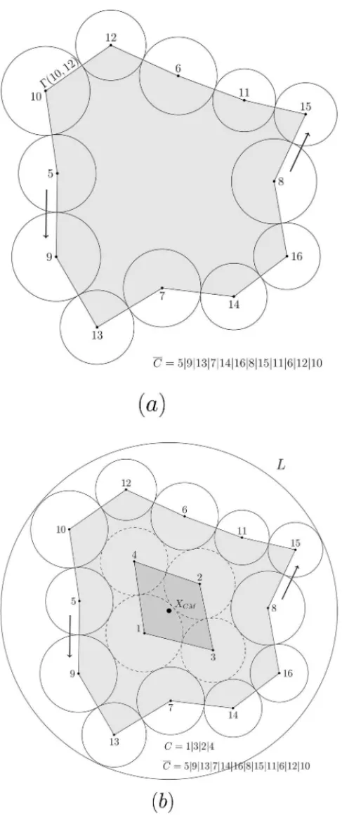
X(i)andX(j). Figure 2(a) illustrates the setŴ(10,12).
Definition 1.(Contact Pair)Ifd(i,j)=ri+rj, we say that{i,j}is aContact Pairof circles.
Definition 2.(Layout)A partialLayout, denoted by L, is a partial pattern (layout) formed by a subset of them 2 of the circle centers, which have already been placed inside the container without overlap. Assume in addition that the container itself is in L. Ifm = n, then L is a complete layout (or solution).
Figure 2(b) illustrates a partial Layout formed by 16 circles placed inside the container. Among others,{5,9}and{8,15}are Contact Pairs.
Definition 3. (Placed Cyclic Order)LetC =i1i2. . .it−1it,ip ∈ N, p =1, . . . ,t, be a cyclic order of circles, which have already been placed inside the container without overlap. In addi-tion, the intersection of any two setsŴ(ip1,iq1)andŴ(ip2,iq2)have at most one endpoint in common, p1,p2,q1,q2∈ {1, . . . ,t}. We say thatCis aPlaced Cyclic Order.
Definition 4. (Contact Cyclic Order)LetCbe a Placed Cyclic Order. If the circles are two by two Contact Pairs inC, we say thatCis aContact Cyclic Order.
Given aC=i1i2· · ·ip−1ipip+1. . .it−1it, we say that the circlesi1,i2, . . . ,ip−1are in counter-clockwiseorder in relation to circleipand the circlesip+1, . . . ,it−1it are inclockwiseorder in relation to circleip.
Definition 5. (Main Area)LetC be a Placed Cyclic Order. We say that the area bounded by the union of the line segmentsŴ(ip,iq), whereip,iqare inC, is theMain AreaofC, which is denoted byA(C).
Figure 2(a) illustrates a Contact Cyclic OrderC¯ formed by 12 circles placed inside the container. Note that all{i,j}inC¯ are two by two Contact Pairs. In Figure 2(b), in addition to C¯, it is illustrated a Contact Cyclic OrderCformed by 4 circles. Note that all circles inC(dashed lines) are completely placed on A(C¯). This is a feature of our approach, since several Contact Cyclic Order are obtained by circling each other. This approach is an important requirement, since it can yield a more compact layout.
LetN¯ ⊂Nbe a subset of circles placed inside the container and| ¯N|be the cardinality ofN¯. We denote thecentroidofN¯ by the coordinatesXC= | ¯N|1
i∈ ¯N
Definition 6. (Border) Let L be a partial Layout and C be a Contact Cyclic Order. If the center of each circle inL belongs toA(C), we say in addition thatCis theBorderof the partial LayoutL.
Figure 2(b) illustrates the BorderC¯ (12 circles) of the partial LayoutL(16 circles). Note that all circle centers inL belong to A(C¯). On the other hand,C =1|3|2|4 is not a Border ofL, since
X(5) /∈ A(C).
We consider two cases of inclusion for placing circles. In the first case, we require that the circle
kto be included must touch at least two previously placed circles. After this, in the second case, we require that another circleℓto be included occupies the wasted spaces after placing the circle
k. This is a reasonable requirement, since it will generally yield a more compact layout than one defined by separate circles.
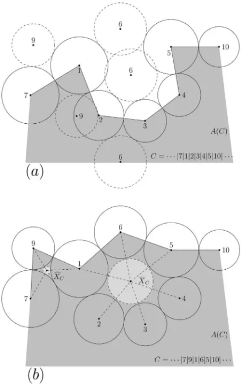
These two cases of inclusion can be explained by a partial Layout of the LOP example with seven existing circles illustrated in Figure 3. In Figure 3(a), it is shown the first case of inclusion. There are two positions to place the circle 9 (dashed lines) touching the Contact Pair{1,7}, and two positions to place the circle 6 (dashed lines) touching the Contact Pair{2,3}. Each position can be obtained by the solutions of the following particular case of the problems of Apolonio (Coxeter, 1968).
⎧ ⎨
⎩
(x−xip)2+(y−yip)2 = rk+rip
(x−xiq)2+(y−yiq)2 = rk+riq
(3)
We denote by St(k,ip,iq)the coordinates of the solution of the System (3) which does not
belongto A(C). Note that the System (3) has two real solutions whenever d(ip,iq) rip +
riq +2rk. In Figure 3(a), by choosingSt(9,7,1)as the coordinates of the circle 9, we obtain a
feasible layout. However, it is not enough to chooseSt(6,2,3)as the coordinates of the circle 6, because the circle 6 overlaps the circles 1 and 5.
In our approach, we always select the coordinatesSt(k,ip,iq) /∈A(C)in order to place the new circlektouching the Contact Pair{ip,iq}in the BorderC (in Figure 3(a), we havek =6 and {ip,iq} = {2,3}), but due to the potentially large differences in the radii, it is possible to occur overlap with the circles in the BorderC. As it is illustrated in Figure 3(a), we get around this situation by repositioning the circlekto the coordinates of the solution of new System (3) fork,
ip¯ andiq¯, where now the circlektouches the circlesip¯ andiq¯ (in Figure 3(b), we havek =6,
ip¯ =1 andiq¯ =5). This first case of inclusion and the possible reposition define the following placement approach.
Definition 7. (External Placement)Let L be a partial Layout andC be the Border of L. An
The External Placement is always selected outsideA(C), however if there is overlap onC, the repositioning of the new circlek(as explained above) is done in the following routine.
Procedure 1: External Placement routine
Input:a circlek, a Contact Pair{ip,iq}, a partial LayoutLand the BorderC Output:an External Placement pE(k), pandq
Step 1.CalculateSt(k,ip,iq)by System (3) andpE(k)←St(k,ip,iq). If the circlekdoes not overlap any circles inCstop, otherwise go to Step 2.
Step 2. While there is overlap between the circle k and the circles inC repeat. If the circle
k overlaps the circleip¯ furthest with respect to the counterclockwise order of the Border C,
p ← ¯p, and if the circlekoverlaps the circleiq¯ furthest with respect to the clockwise order of the BorderC,q ← ¯q, and choose pE(k)as the solution of the System (3) that is furthest from the centroid of the circles inLwith respect to the Euclidean distance.
First, if the new circlekdoes not overlap any circles in BorderC, the External Placement routine selects pE(k) = St(k,ip,iq). In our approach, this case is the most convenient way to place the next circle. However, if there is overlap, in Step 2 the routine identifies such circles (ip¯ and
iq) in order to reposition the circle¯ kfurther from the centroid of the partial Layout, eventually avoiding any kind of overlap.
To obtain a more compact layout, after including the circlek, it is checked the possibility of including another circle to occupy the wasted spaces after placing the circlek. We check among the remaining circles outside the container (preferably the largest one) if there is a circleℓthat can be placed into the container in a centralized position without overlap. Each centralized position is the centroid coordinates of a certain set of circles which includes the circle k and the two circles touching the circlek. Figure 3(b) illustrates the second case of inclusion, which we can investigate the possibility of positioning a circle in the wasted space after placing the circle 9 touching the Contact Pair{1,7}(centroid XˆC of the circles{1,7,9}), and in the wasted space after placing the circle 6 touching the circles 1 and 5 (centroidX¯Cof the circles{1,2,3,4,5,6}).
Definition 8.(Internal Placement). LetL be a partial Layout,Cbe the Border ofL, and{ip,k}, {k,iq}be Contact Pairs inC, wherekis the previous circle included. AnInternal Placementis the placement of a circleℓinside the container, so that its center belongs to A(C), ℓdoes not overlap with any other circle, and the center of ℓis placed at the centroid coordinates of the subset N¯, where{k,ip,iq} ⊆ ¯N. We denote an Internal Placement bypI(N¯, ℓ), meaning thatℓ is to be placed at the centroid coordinatesXCofN¯.
Figure 3–Two cases of inclusion: (a) External Placement and (b) Internal Placement.
placement of the circlekcauses the addition of one element inLand one index inC, and perhaps the removal of some indices fromC. This will be represented by the following operation.
O−+(k,ip,ip+s)(C)=C+ {k} − {ip+1, . . . ,ip+s−1} =i1i2· · ·ipk ip+s· · ·it−1it,
where 1s ⌊(t−2)/2⌋.
With this choice forsthere are fewer indices betweenpandp+sthanp+sand p.
The possible placement of the circleℓafter the placement of the circlekonly causes the possible addition of the coordinatesX(ℓ)to the partial LayoutL.
In our approach, we require the imbalance of the system be zero. It seems intuitive that this requirement may result in a good solution. We denote the center of mass of the system by
XC M =(xC M,yC M)=(1/ n
i=1 mi)
n
i=1 mixi,
n
i=1 miyi
,
then one can shift the center of the rotating circular container to the center of mass of the system to have zero imbalance. This shift is made at eachouter iterationand at the end of the algorithm, but it may increase the envelopment radius. Thus, if the LayoutLrepresents a complete solution of the LOP, we denote the radiusrof the container by
r =R(L)≡ max
1kt
rik +d(XC M,X(ik))
.
Moreover, the index whereR(L)is reached is denoted bykmax≡arg(R(L)).
3 CENTER-OF-MASS-BASED PLACING TECHNIQUE (CMPT)
We present a new placing technique which yields compact layouts and quality solutions in an efficient manner. Letα = (α(1), α(2), . . . , α(n))be a permutation of(1,2, . . . ,n). We place the circles in the partial LayoutL one by one according to the order defined by this permutation. Given a order of inclusion, the first circles α(1), α(2), α(3)and α(4)must be positioned as follows.
Procedure 2: Initial layout routine
Input:the circlesα(1),α(2),α(3)andα(4)
Output:an initial LayoutLand the initial BorderC
Place the circleα(1)at coordinates X(α(1)) = (0,0). Choose the coordinates X(α(2)), such thatα(2)touchesα(1). For each circleα(3)andα(4), solve the System (3) and place them at co-ordinatesX(α(3))=(xα(3),yα(3))=St(α(3), α(1), α(2))andX(α(4))=St(α(4), α(1), α(2)) without overlap.L = {X(α(1)),X(α(2)), X(α(3)),X(α(4))}andC←α(1)|α(3)|α(2)|α(4).
Figure 2(b) illustrates the initial L = {X(1),X(2),X(3),X(4)} and the initial BorderC = 1|3|2|4. Among many optional positions we can chooseX(α(2)), for example, at thex-axis with the coordinates(rα(1)+rα(2),0).
When we place the circleα(k)(wherek>4, see Procedure 2), we require that the circle touches at least two previously placed circles (see Figure 3(a) and Procedure 4). This will generally yield a more compact layout. However, we can increase the compactness of the layout if the wasted spaces after placing the circleα(k)can be occupied by another circleα(ℓ)(see Figure3(b) and Procedure 4).
We observe that for each additional circle, the envelopment radius of a layout is generally en-larged. In order to minimize the rate of growth of this radius during inclusions, we must properly choose a new position for circleα(k)which yields a smaller envelopment radius. Our strategy CMPT attempts to reduce the rate of growth of the envelopment radius by including every circle around the coordinates of the center of mass of the system, which is updated during each outer iteration.
This strategy consists of shifting the origin of the Euclidean plane to the current center of mass of the system. Then we require that the circleα(k)touches the circles of a Contact Pair arbitrar-ily chosen among the elements of the BorderC, taking into consideration the quadrants of the Euclidean plane. This approach is performed according to the following routine.
Procedure 3: CMPT routine
Input:a partial LayoutL and the BorderC Output:the setsQ1,Q2,Q3andQ4
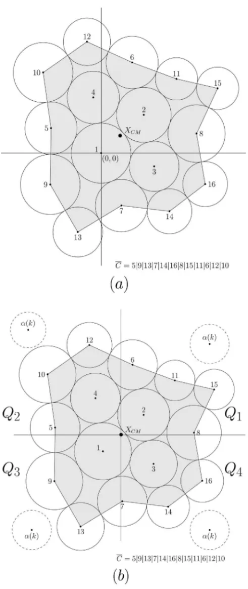
Step 1.Calculate the coordinates of the center of massXC M of the circles inL, and translate the origin of the Euclidean plane toXC M.
Step 2.Include each Contact Pair{ip,ip+1}ofCin the setQhif the center ofipbelongs to the quadranthof the Euclidean plane, forh=1,2,3,4.
Given the BorderC, the Procedure 3 only separates the Contact Pairs inC according to the quadrants of the Euclidean plane with origin shifted to the current center of mass of the system.
Figure 4 illustrates the Procedure 3. In Figure 4(a) we observe that the coordinates of the center of massXC M of the system do not coincide with the coordinates of the originX(α(1))=(0,0). We wish to place the next circleα(k)around the coordinates XC M in order to mitigate the growth of the envelopment radius. By dividing the plane into quadrants, we can obtain a BorderC
with a more circular shape. We see in Figure 4(b) that if we place each new circleα(k) at a different quadrant of the Euclidean plane (with the origin shifted toXC M), then the layout is more evenly distributed.
Next we describe the two cases of inclusion in the following routine.
Procedure 4: Inclusion routine
Input:a circleα(k), a permutationα, the setsQh,h=1,2,3,4, a Contact Pair{ip,iq}in a set
Qh, a partial LayoutLand the BorderC
Output:a partial LayoutL, the BorderC and the setsQh,h =1,2,3,4
Step 1. Obtain an External Placement pE(α(k))and the new values for pandq by Procedure 1. If there are fewer indices in the BorderCbetweenq andpthan those between pandq, then
¯
p← p,p←qandq← ¯p.
Step 2.C← O−+(α(k),ip,iq)(C),X(α(k))← pE(α(k)),L ← L∪{X(α(k))}andQh← Qh\
{ip,ip+1}, . . . ,{iq−1,iq},h=1,2,3,4 (note thatq= p+s, where 1s⌊(t−2)/2⌋).
Step 3. If it is possible to obtain an Internal Placement pI(N¯, α(ℓ))for the set N¯ = {α(k),ip,
ip+1, . . . ,iq−1,iq}and a circleα(ℓ)(preferably the largest) in the permutationα,k < ℓ n, thenX(α(ℓ))← pI(N¯, α(ℓ)),L← L∪ {X(α(ℓ))}, and excludeα(ℓ)fromα.
The Inclusion routine attempts to place the new circles in a more compact layout. First, it com-putes an External Placement for the next circleα(k)by Procedure 1 and updates the values forp
andqin order to obtain fewer indices betweenpandqthan those betweenqandp. In Step 2, the BorderCis updated by the operationO−+, where the indices between pandq are removed from
C(by Step 1, those indices correspond to the internal circles from the Border when compared to the indices betweenq and p), andα(k)is added toC. The circleα(k)is placed inside the con-tainer and all Contact Pairs between pandq (including{ip,ip+1}and{iq−1,iq}) are removed from the sets Qh, h = 1,2,3,4. This choice guarantees that the operation O−+will exclude the internal circles from the BorderC. Finally, a search to place another circleα(ℓ) (Internal Placement) is performed.
Post-optimization
A post-optimization is performed after the algorithm builds a complete solution (represented by Layout L), which contemplates improvements via circle repositioning at the Border C of L. This post-optimization process causes changes inC, where an index is removed and then it is repositioned inCby operationO−+. The removal of the index fromCwill be represented by the following operation.
D(ip)(C)=i1i2· · ·ip−1ip+1· · ·it−1it.
Main routine
We choose to position each circle inside the container according to the following main procedure.
Main routine
Input:a permutationα=(α(1), α(2), . . . , α(n)) Output:a LayoutL(complete solution)
Step 1. (Initialization) Obtain the initial Layout L and the initial BorderC by Procedure 2,
k←5.
Step 2.(CMPT) Obtain the setsQh,h=1,2,3,4 by Procedure 3.
Step 3. (Layout construction) While there are Contact Pairs in any Qhand circles outside the container, repeat for eachh =1,2,3,4.
IfQh = ∅, choose an arbitrary{ip,iq} ∈ Qhand include the circleα(k)and the possible circleα(ℓ),k< ℓn, by Procedure 4 andk←k+1.
Step 4.If there are circles outside the container, return to Step 2. Otherwise, go to Step 5.
Step 5.(Post-optimization)L¯ ← L,C¯ ←C,r¯←R(L¯), computekmaxinC¯ andk←kmax. Step 5.1. (x¯,y¯) ← X(ik), delete the current X(ik)and repeat Step 5.2. for each Contact Pair {ip,iq}ofC¯, excluding{ik−1,ik}and{ik,ik+1}.
Step 5.2. Obtain an External Placement pE(ik)and the new values for p andq by Procedure 1, and X(ik) ← pE(ik). If the radius of the container is improved, then C¯ ← D(ik)(C¯),
¯
C ←O−+(ik,ip,iq)(C¯),L ← ¯L,C← ¯Cand return to Step 5.
Step 5.3. X(ik) ← (x¯,y¯)and finish the routine with the complete solutionL ← ¯L, whose container center is the center of mass of the system.
Given a permutationα, the Main routine builds an initial Layout Lin Step 1 by placing the first four circles as in Procedure 2. Next, in Step 2 the main aspect of our approach is performed by Procedure 3 (CMPT routine), where the Euclidean plane is divided into four parts and the subsets
Qh (h =1,2,3,4) of Contact Pairs are obtained. Next, Step 3 is repeated by looking at each subset Qhand while there are circles remaining to be placed. In this step, an arbitrary Contact Pair inQh is chosen and the two cases of inclusions are performed by Procedure 4. After we finish placing all circles inside the container, we obtain a complete solutionL and its Border
Order of placement of the circles
As previously described, a permutationα=(α(1), α(2), . . . , α(n))of(1,2, . . . ,n)is used as an input in our algorithm to generate a layout by specifying the order in which the circles are placed. Since there existn!possible permutations forncircles, we need an appropriate technique in order to search in such a large space. Preliminary tests show that the wasted spaces after placing circles are minimized with greater efficiency when the order of addition of the circles favors those of larger radii.
Letα=(α(1), α(2), . . . , α(n))be a sequence obtained by considering their radii in descending order of the circles, i.e., rα(k) rα(j), 1 k < j n. Choose an integerb, 1 b n and subdivide the terms of the sequenceαinℓ= ⌊n/b⌋blocks. Thus, it is possible to obtain a subsequenceα¯ofαto be used as an input to the algorithm, by permuting the positions of the first α(1), . . . , α(ℓ)elements ofα, theα(ℓ+1), . . . , α(2ℓ)elements ofα, and so on, until we permute the positions ofα(bℓ), . . . , α(n−1), α(n)last elements ofα. With this procedure, several sub-sequences to place the different circles may be generated. Actually, there are((ℓ!)b)(n−(bℓ))! possibilities, so that 1((ℓ!)b)(n−(bℓ))!n!. Thus, whenb=n, we only obtain the sequence
¯
α = α, and whenb =1, we can generate at mostn!distinct subsequences. In our numerical experiments, for each instance of dimension greater than or equal to 10 we chose b = 5 to generate such sequences.
Complexity
The analysis of the real computational time of the Main routine is difficult, because it does not depend only on the number of circles, but also on the diversity of the circle radii and the number of circles in a current BorderC, as well as the implementation. Here, we analyze the upper bound of the complexity of the Main routine, when it finds a complete solutionL with BorderC, such that|C| = λn, where 0< λ 1, including the post-optimization process. Recall that, before post-optimization, the circles in BorderCare two by two Contact Pair.
Given a partial Layout L withm circles already placed inside the container andn−mcircles outside. Let|C|be the number of circles in the BorderCof the partial LayoutL.
The strategy CMPT in Procedure 3 checks the position of|C| circles in the Euclidean plane, which is done inO(|C|).
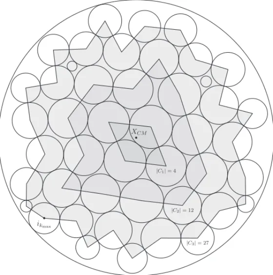
|C3|= 27 1
|C2|= 12
|C1|= 4
• ikmax
• XCM
Figure 5–A suboptimal solution: 45 circles inside the container.
After placing the circleik, we must check if there is a circleiℓoutside the container to be placed in an Internal Placement, then we must check the overlaps amongn−mcircles and a subset N¯
inC, which is done in about| ¯N| ×(n−m)|C| ×(n−m).
In the post-optimization process, we select one circle inCand assess at most(|C| −2)Contact Pairs inCto try to improve of the envelopment radius by checking at most 2×(|C| −2)External Placements, thus the complexity of the post-optimization is bounded by 2×(n−1)×(|C| −2).
Therefore the complexity of placingn circles during the Main routine is bounded byO(n2|C|). After placing the new circleik, the operationO−+modifies the BorderC. This operation controls the size ofC during the iterations. Since|C|n, the theoretical upper bound isO(n3).
4 EXPERIMENTAL RESULTS
series of heuristics based on energy landscape paving, gradient method and local search (Liu & Li, 2010; Liu et al. 2010, 2015), and a series of algorithms based on quasi-physical approaches, gradient method and local search (Huang & Chen, 2006; He et al. 2013; Liu et al. 2015).
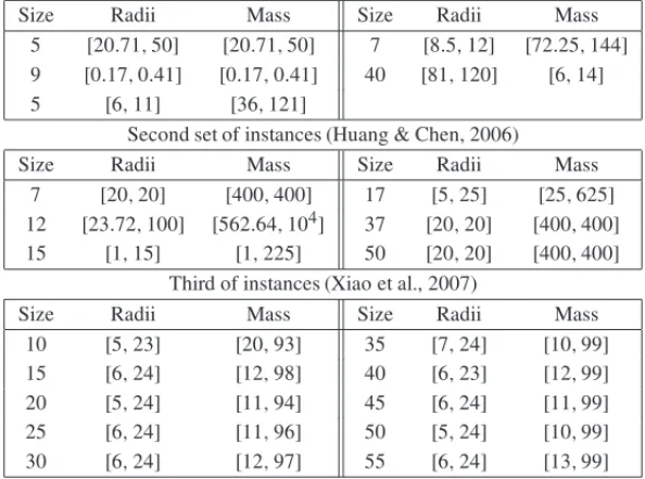
Table 1–Data of each instance. First set of instances (Liu & Li, 2010).
Size Radii Mass Size Radii Mass
5 [20.71,50] [20.71,50] 7 [8.5,12] [72.25,144] 9 [0.17,0.41] [0.17,0.41] 40 [81,120] [6,14] 5 [6,11] [36,121]
Second set of instances (Huang & Chen, 2006)
Size Radii Mass Size Radii Mass
7 [20,20] [400,400] 17 [5,25] [25,625] 12 [23.72,100] [562.64,104] 37 [20,20] [400,400] 15 [1,15] [1,225] 50 [20,20] [400,400]
Third of instances (Xiao et al., 2007)
Size Radii Mass Size Radii Mass
10 [5,23] [20,93] 35 [7,24] [10,99]
15 [6,24] [12,98] 40 [6,23] [12,99]
20 [5,24] [11,94] 45 [6,24] [11,99]
25 [6,24] [11,96] 50 [5,24] [10,99]
30 [6,24] [12,97] 55 [6,24] [13,99]
These methods search for the optimal layout by directly evolving the positions of every circle, as well as considering imbalance. We use the benchmark suite of 21 instances of the problem described in Table 1 to test our algorithm. For each instance we present the range forri and
mi. A more detailed description of the instances can be found in Huang & Chen (2006), Liu & Li (2010) and Xiao et al. (2007).
The routines were implemented in MATLAB language, and executed on a PC with an Intel Core i7, 7.7 GB of RAM and Linux operating system.
Except for the instances 1.1 and 1.3, both of them with 5 circles, we decide to generate 7! =5040 distinct permutationsαas input for the algorithm in each instance, i.e., we fixed in 5040 the number of executions of the Main routine for each instance and the best solution found was selected. This amount of tests proved adequate for our comparisons.
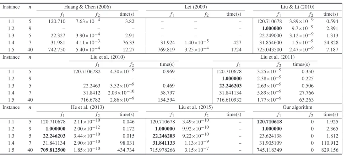
The results from the first, second and third sets of instances are presented in Tables 2, 3 and 4 respectively, where we compare our approach with those described in each indicated reference. The results are shown for the size of the instances, the best radius of the container obtained (first objective function f1), the imbalance obtained (second objective function f2), and the running
Table 2 shows that our approach proved to be competitive. We obtained the best value for f1on
instance 1.1, tied in instance 1.2, while obtained results 6.1%, 0.2% and 4.0% worse than the best result on instances 1.3, 1.4 and 1.5 respectively.
Similar results were obtained in the second set test, as can be seen in Table 3. Our algorithm tied in instance 2.1 and 2.2, while obtained results at most 7.7% worse than the best result on instances 2.3, 2.4, 2.5 and 2.6.
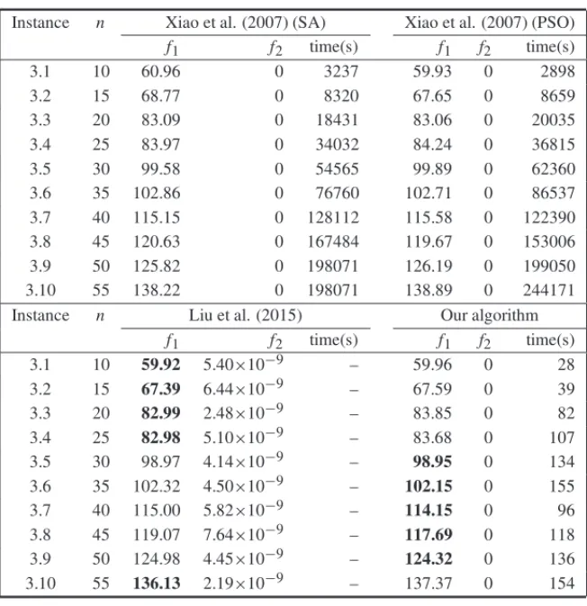
In Table 4 we compare our approach with three other algorithms. The first set of data are from a version of simulated annealing (SA), the second set of data are from the same reference, but one of them is a version of particle swarm optimization (PSO), while the third set of data is a heuristic based on energy landscape paving. Again, our approach proved to be competitive. In relation to the envelopment radius we obtained better results in 5 out of the 10 instances. We only obtained worse results in five cases, but they were on average approximately 0.63% worse than the results from literature for such instances.
Overall, running time obtained by our algorithm can be considered good. Since the center of the rotating circular container is shifted to the center of mass of the system we always have f2=0,
making our solutions more interesting than the others for this first set of instances.
Figure 5 illustrates a typical solution obtained by our algorithm for an instance of 45 circles. Note that the large BorderC3have 27 circles, i.e., 60% of the size, and when we carefully read the CMPT routine, we can see that the initial BorderC1(|C1| =4) is iteratively transformed in
the BorderC2(|C2| =12), and finally the latter is iteratively transformed in the BorderC3. In this example there were only two inclusions by Internal Placement.
The computational results show that the proposed algorithm is an effective method for solving the circular packing problem with additional balance constraints.
5 CONCLUSIONS
We have presented a new heuristic called center-of-mass-based placing technique for packing unequal circles into a 2D circular container with additional balance constraints. The main feature of our algorithm is the use of the Euclidean plane with origin in the center of mass of the system to select a new circle to be placed inside the container. We evaluate our approach on a series of instances from the literature and compare with existing algorithms. The computational results show that our approach is competitive and outperforms some published methods for solving this problem. We conclude that our approach is simple, but with high performance. Future work will focus on the problem of packing spheres.
ACKNOWLEDGEMENTS
IN G T O N A. D E O L IVEI R A, L U IZ L . D E SAL L ES N ET O , AN T O N IO C . M O R ET T I a n d ED N EI F . R EI S
Table 2–Numerical results for the first set of instances
Instance n Huang & Chen (2006) Lei (2009) Liu & Li (2010)
f1 f2 time(s) f1 f2 time(s) f1 f2 time(s)
1.1 5 120.710 7.63×10⁻⁴ 3.82 – – – 120.710678 3.89×10⁻⁹ 0.594
1.2 9 – – – – – – 1.000000 9.7×10⁻⁹ 2.891
1.3 5 22.327 3.90×10⁻⁴ 2.91 – – – 22.249000 3.12×10⁻⁹ 1.313
1.4 7 31.981 4.11×10⁻³ 76.33 31.924 1.40×10⁻⁵ 427 31.854600 1.5×10⁻⁹ 54.828
1.5 40 742.750 5.40×10⁻⁴ 12.27 769.819 3.25×10⁻⁴ 1724 725.043500 2.47×10⁻⁹ 7.187
Instance n Liu et al. (2010) Liu et al. (2011)
f1 f2 time(s) f1 f2 times(s)
1.1 5 120.7106782 4.30×10⁻⁹ 0.969 120.710678 3.25×10⁻⁹ 0.350
1.2 9 – – – 1.000000 2.38×10⁻⁹ 0.225
1.3 5 22.2463 3.52×10⁻⁹ 0.469 22.246203 2.63×10⁻⁹ 0.506
1.4 7 31.8412 2.03×10⁻¹⁰ 58.797 31.841134 5.89×10⁻⁹ 27.766
1.5 40 716.6782 2.86×10⁻⁹ 154.594 716.610932 1.77×10⁻⁹ 63.263
Instance n He et al. (2013) Liu et al. (2015) Our algorithm
f1 f2 time(s) f1 f2 time(s) f1 f2 time(s)
1.1 5 120.710678 2.11×10⁻¹⁰ 0.046 120.710678 3.49×10⁻¹⁰ – 120.710618 0 1.925
1.2 9 1.000000 2.00×10⁻¹² 0.172 1.000000 9.92×10⁻¹⁰ – 1.000000 0 2.365
1.3 5 22.246203 3.44×10⁻¹⁰ 0.015 22.246203 9.22×10⁻¹⁰ – 23.624138 0 1.812
1.4 7 31.841134 2.90×10⁻¹⁰ 98.031 31.841133 1.13×10⁻⁹ – 31.905109 0 110.912
1.5 40 709.812500 1.85×10⁻¹⁰ 434.734 715.978266 3.15×10⁻⁷ – 745.118349 0 829.156
A N E W HE URIS T IC A L G O R IT HM F O R T HE B A L A NCE CO NS T R A INT S C A S
E Table 3–Numerical results for the second set of instances
Instance n Huang & Chen (2006) Liu et al. (2010) Liu et al. (2011)
f1 f2 time(s) f1 f2 time(s) f1 f2 time(s)
2.1 7 60.00 3.6×10⁻³ 7.78 60.0000 1.59×10⁻⁹ 1.031 60.000000 7.38×10⁻⁹ 0.206 2.2 12 215.470 9.5×10⁻³ 444.78 215.470054 2.74×10⁻⁷ 11.562 215.470054 3.77×10⁻⁷ 3.042 2.3 15 39.780 7.6×10⁻³ 91.92 39.123400 2.97×10⁻⁸ 130.362 39.065105 4.13×10⁻⁸ 365.797 2.4 17 49.720 5.1×10⁻³ 157.92 49.507800 6.83×10⁻⁸ 123.407 49.368194 2.50×10⁻⁸ 597.719 2.5 37 135.176 6.7×10⁻³ 18.29 135.175410 1.23×10⁻⁸ 0.203 135.175410 4.91×10⁻⁹ 0.425 2.6 50 159.570 8.0×10⁻³ 348.97 158.967800 4.81×10⁻⁹ 453.625 158.967698 3.49×10⁻⁹ 1078.386
Instance n He et al. (2013) Liu et al. (2015) Our algorithm
f1 f2 time(s) f1 f2 time(s) f1 f2 time(s)
2.1 7 60.000000 2.66×10⁻⁹ 0.015 60.000000 5.13×10⁻⁹ – 60.000000 0 0.118
2.2 12 215.470054 2.92×10⁻⁸ 0.391 215.470054 1.69×10⁻⁷ – 215.470054 0 52.125
2.3 15 39.037635 7.78×10⁻¹⁰ 36.343 39.065105 1.12×10⁻⁸ – 40.090538 0 167.248
2.4 17 49.338750 1.51×10⁻⁹ 10.562 49.368194 1.42×10⁻⁸ – 50.246873 0 325.080
2.5 37 135.175410 6.95×10⁻⁹ 0.234 135.175410 3.35×10⁻⁹ – 145.624231 0 0.402
2.6 50 158.963672 5.14×10⁻⁹ 268.078 158.967698 3.65×10⁻⁹ – 163.206698 0 0.390
Table 4–Numerical results for the third set of instances
Instance n Xiao et al. (2007) (SA) Xiao et al. (2007) (PSO)
f1 f2 time(s) f1 f2 time(s)
3.1 10 60.96 0 3237 59.93 0 2898
3.2 15 68.77 0 8320 67.65 0 8659
3.3 20 83.09 0 18431 83.06 0 20035
3.4 25 83.97 0 34032 84.24 0 36815
3.5 30 99.58 0 54565 99.89 0 62360
3.6 35 102.86 0 76760 102.71 0 86537
3.7 40 115.15 0 128112 115.58 0 122390
3.8 45 120.63 0 167484 119.67 0 153006
3.9 50 125.82 0 198071 126.19 0 199050
3.10 55 138.22 0 198071 138.89 0 244171
Instance n Liu et al. (2015) Our algorithm
f1 f2 time(s) f1 f2 time(s)
3.1 10 59.92 5.40×10⁻⁹ – 59.96 0 28
3.2 15 67.39 6.44×10⁻⁹ – 67.59 0 39
3.3 20 82.99 2.48×10⁻⁹ – 83.85 0 82
3.4 25 82.98 5.10×10⁻⁹ – 83.68 0 107
3.5 30 98.97 4.14×10⁻⁹ – 98.95 0 134
3.6 35 102.32 4.50×10⁻⁹ – 102.15 0 155
3.7 40 115.00 5.82×10⁻⁹ – 114.15 0 96
3.8 45 119.07 7.64×10⁻⁹ – 117.69 0 118
3.9 50 124.98 4.45×10⁻⁹ – 124.32 0 136
3.10 55 136.13 2.19×10⁻⁹ – 137.37 0 154
REFERENCES
[1] COXETERHSM. 1968. The problem of Apollonius.The American Mathematical Monthly,75(1): 5–15.
[2] HEK, MOD, YET & HUANGW. 2013. A coarse-to-fine quasi-physical optimization method for solving the circle packing problem with equilibrium constraints.Computers & Industrial Engineer-ing,66(4): 1049–1060.
[3] HUANGW & CHENM. 2006. Note on: An improved algorithm for the packing of unequal circles within a larger containing circle.Computers & Industrial Engineering,50(3): 338–344.
[4] LEIK. 2009. Constrained layout optimization based on adaptive particle swarm optimizer. Springer-Verlag Berlin Heidelberg,1: 434–442.
[6] LIN, LIUF & SUND. 2004. A study on the particle swarm optimization with mutation operator constrained layout optimization.Chinese Journal of Computers (in Chinese),27(7): 897–903, apud in XIAORB, XUYC & AMOSM (2007).
[7] LIUJ, JIANGY, LIG, XUEY, LIUZ & ZHANGZ. 2015. Heuristic-based energy landscape paving for the circular packing problem with performance constraints of equilibrium.Physica A: Statistical Mechanics and its Applications,431: 166–174.
[8] LIUJ & LIG. 2010. Basin filling algorithm for the circular packing problem with equilibrium be-havioral constraints.Science China Information Sciences,53(5): 885–895.
[9] LIUJ, LIG, CHEND, LIUW & WANGY. 2010. Two-dimensional equilibrium constraint layout using simulated annealing.Computers & Industrial Engineering,59(4): 530–536.
[10] LIUJ, LIG & GENGH. 2011. A new heuristic algorithm for the circular packing problem with equilibrium constraints.Science China Information Sciences,54(8): 1572–1584.
[11] QIANZ, TENGH & SUNZ. 2001. Human-computer interactive genetic algorithm and its application to constrained layout optimization.Chinese Journal of Computers,24(5): 553–560, apud in XIAO
RB, XUYC & AMOSM (2007).
[12] TANGF & TENGHF. 1999. A modified genetic algorithm and its application to layout optimization.
Journal of Software (in Chinese),10: 1096–1102, apud in XIAORB, XUYC & AMOSM (2007). [13] TENGHF, SUN SL, GEWH & ZHONGWX. 1994. Layout optimization for the dishes installed
on rotating table – the packing problem with equilibrium behavioural constraints.Science in China Mathematics (Series A),37(10): 1272–1280.
[14] WANGH, HUANGW, ZHANGQ & XUD. 2002. An improved algorithm for the packing of unequal circles within a larger containing circle.European Journal of Operational Research,141(2): 440– 453.
[15] XIAORB, XUYC & AMOSM. 2007. Two hybrid compaction algorithms for the layout optimization problem.Biosystems,90(2): 560–567.
[16] XUYC, XIAORB & AMOSM. 2007. A novel genetic algorithm for the layout optimization problem. In: ‘Evolutionary Computation, 2007. CEC 2007. IEEE Congress on’, IEEE, pp. 3938–3943. [17] ZHOUC, GAO L & GAO H. 2005. Particle swarm optimization based algorithm for constrained