Abstract – This paper proposes an approach to estimate the probable location of maximum exposure to electromagnetic fields associated with a radiocommunication station, based only on information of antenna’s height, half-power angle and tilt. This approach can be implemented when simulation tools are absent, or/and few basic information on radiating system is available. The proposed analytical expression is compared with simulated and real measured data, showing the good accuracy of the proposed technique. The focus of the work are base stations, however the results may be applicable to any radiocommunication station. As far as the authors know, this is the first study to present a mathematical formulation in closed form under the considered constraints.
Index Terms – Antenna, electromagnetic field, human exposure, radiocommunication station.
I. INTRODUCTION
The proliferation of radio base stations in urban environments has raised a worldwide public concern regarding electromagnetic fields (EMF). National authorities are facing the challenges to conciliate public demands, local authorities’ restrictive laws and the need to develop a regulatory framework to guarantee the efficient development of the mobile telephony network. In response to such concern, international bodies are constantly developing studies, recommendations and standards to serve as guidelines on how to manage EMF exposure.
The issue of human exposure to EMF can have two different approaches. The first one can be treated from the perspective of possible adverse health effects and, the second, from the perspective of the electromagnetic environment characterization. For the first one, the World Health Organization (WHO), together with the International Commission for Protection on Non-Ionizing Radiation Protection (ICNIRP) and the Institute of Electrical and Electronics Engineers (IEEE) develop studies to establish exposure limits and evaluate the biological effects of those exposures. For the second approach, the IEEE, as well as the International Electrotechnical Commission (IEC), and the International Telecommunications Union (ITU) develop standards and recommendations to characterize the environment and evaluate the compliance of exposure limits [1].
International standards and recommendations address exposure assessment in two ways: the first and simplest one considers only theoretical calculations, while the second considers the field measurements.
Agostinho Linhares, Marco Antonio Brasil Terada and Antonio José Martins Soares
Antenna Group, Electrical Engineering Dept., University of Brasilia – DF, Zip Code 70.910-900 [email protected], [email protected] and [email protected]
Estimating the Location of Maximum Exposure
to Electromagnetic Fields Associated with a
Regarding the theoretical calculations, it is desirable to have the knowledge of all installation parameters. However some simplifications are possible and the necessity of refinement is proportional to the EMF level in the vicinity of the station being evaluated. For instance, just knowing the equivalent isotropically radiating power (EIRP) and antenna height may be sufficient if the EMF level is low compared with the compliance limit.
Regarding the field measurements the evaluation can be classified as broadband or narrowband (or selective). The broadband measurement provides a quick overview of the overall EMF levels, without taking into account the individual source (frequency) contributions. The narrowband or selective measurement provides a detailed investigation of the individual source contributions and then the multiple frequencies EMF levels.
Having the knowledge of the radiating system parameters, such as antenna height, half-power angle and tilt is important for any evaluation on the field. Moreover, for broadband measurements, it is important to know about the traffic characteristics; for instance, if the measurement is being recorded in peak, use hour. For the narrowband evaluation, technology information, such as the signal bandwidth, modulation type and medium access techniques are relevant to enable the correct configuration of measurement systems. Other information like antenna gain and EIRP are also desirable.
Both methods, theoretical calculations or field measurements, have advantages and disadvantages. Some advantages of the former are the possibility of simulating non existing radiating sources, the possibility to take into account the maximum possible EIRP, simulation of mitigation techniques before installation, calculation in areas with no access; while some disadvantages are that very accurate results require detailed description of the radiating antennas and environment, and also in most cases do not take into account the influence of reflections [2].
On the other hand, some advantages of fields measurements are that it takes into account all radiating sources with real parameters and the real environment, including reflections, antenna supporting hardware, obstacles, and waves’ phase differences and the evaluation can be done with little knowledge about sources (although it desirable initial measurement of the occupied spectrum). Nevertheless, some disadvantages are that the effect of the surveyor presence (body reflections) has to be avoided, checking if all sources are operating in maximum EIRP is difficult and post-processing may be applicable [2].
One of the key points to ensure a proper assessment of human exposure to EMF is the careful selection of measurement points. In some technical standards there are general comments as in [3] [4], including the specification of minimum distances, where higher distances inherently complies the limit [5] [6]. However, the assessment should consider all relevant sources, which can be installed in different locations.
This paper proposes a mathematical formulation in closed form to estimate the location of maximum exposure, due to a radiating system, considering the following installation parameters: antenna height, half-power angle diagram (vertical) and tilt. This approach can be used in case of lack of simulation tool or unknown radiating diagram, taking into account usual installation information, and can be very useful for surveyors that are on the field evaluating a radiocommunication station already in operation.
II. CHARACTERIZATION OF ELECTROMAGNETIC ENVIRONMENT DUE TO BASE STATIONS
purpose of this work deals with EMF exposure not EMF coverage, the proposed model captures the primary impact of path loss, representing a first-order approximation of maximum exposure to EMF associated with a radiocommunication station, giving guidance for technical staff that must check in situ the location of maximum exposure.
The two-ray model is a simplification of the ray tracing method and may be used when a single ground reflection dominates the multipath effect. The person being exposed will receive an E-field consisting of two components, the line of sight (LOS) component, which is the transmitted signal propagating through free space, and a non-line of sight (NLOS) component, which is the transmitted signal reflected off the ground. Moreover, the reflected E-field is proportional to the direct E-field, by a complex factor Γ (reflection coefficient), that has amplitude and phase. The complex Γ depends on the signal wavelength, polarization, surface’s permittivity and conductivity and incidence angle of the reflected ray.
For distances smaller than a critical distance, the composite signal presents a sequence of constructive and destructive interference, resulting in a wave pattern with local maxima and minima (fast fading mechanism). This critical distance can be approximated by the fourfold of the product between the transmitting antenna height and the receiver point height, divided by the wavelength [7].
It is important to note that the decaying behavior of the signal power density in the two-ray model can be approximated by averaging out its local maxima and minina, resulting in a 20 dB/decade power density decaying for distances smaller than the critical distance [7]. In short, discounting the moving average of a two-ray approach will present a result compatible with a free space condition model. For a conservative approach, once exposure to EMF is not only an engineering issue, but also a health protection issue, the reflection coefficient should be considered as an absolute value and reflected signal in-phase with the direct signal.
Macrocell base station antennas are usually installed with a downward tilt, which can be a mechanical, electrical or both. Without the tilt, most of the power density radiated from the antennas would be spread out without reaching the mobile telephone users.
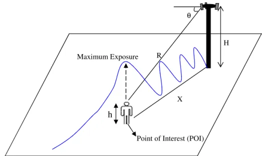
Usually, the maximum exposure to EMF associated to a base station is due to the main beam of the antenna and is located in the range of some tens to a few hundred meters from its mast. Considering the ground level, exposure in distances closer to the base station are usually associated with side lobes that transport less energy than the main beam [5][8][9][10]. Figure 1 presents this signal behaviour graphically.
Figure 1 – The blue line shows the E-field intensity along the azimuth direction of the sector antenna. There are local peaks due to antenna sidelobes closer to the mast, however the maximum exposure tends to occur in a farther
location, and from this point on, the power density decreases monotonically with distance.
Usually, this maximum exposure will occur in the azimuth direction between:
< < (1a)
( ) < < ( ) (1b)
Where:
= ( ), is the point “illuminated” by the first null of the antenna below the horizon. From
this point on, the exposure increases until reaching the maximum;
= ( ), is the point “illuminated” by the antenna’s maximum radiation;
H is the height of the antenna;
h is the reference height where measurement are done;
α is the antenna tilt, i.e., the angle between the maximum radiation direction and the horizon;
is the first null of the antenna below the horizon; and
is the point where a person would be exposed to a maximum power density associated with the emission of the source being evaluated, taking into account only the main lobe.
The parameter h represents a citizen’s average height, but must be understood as an observation point height h, which means that if the evaluation is being done on the top of a building, h will be the building height plus the average height of a citizen.
H
θ
R
X
Point of Interest (POI) Maximum Exposure
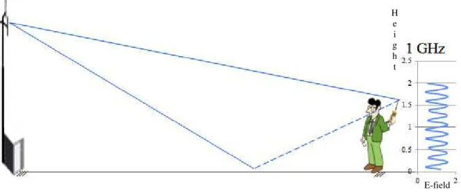
Additionally, it has to be noted that the whole body is passive to EMF exposure, so to minimize multipath reflections an averaging process1 is recommended, as presented in [3][12]. Figure 2 presents a scenario that follows the two-ray model for distances smaller than the critical distance. The E-field intensity variation for a 1 GHz signal along a whole body will have local peaks and valleys, but for a medium size person the mean E-field intensity tends to converge to the direct signal level.
Figure 2 – The mean E-field intensity tends to converge to a reference value E, but considering |Γ| = 0.6 there will be local peaks of 1.6 × E and local valleys of 0.4 × E. The y-axis represents the
height in meter and the x-axis represents the field in relation to a reference value E.
The range of maximum exposure presented in equations (1a) and (1b) represents the region where the antenna’s main lobe reaches the height h. This region is bounded taking into account the antenna’s first null, , plus the tilt, α, and the angle of maximum radiation, which in this case is α. It is important to note that depending upon the antenna’s tilt, the maximum exposure can occur closer to the base station due to the side lobes.
Figure 3 – The maximum exposure, usually, occurs in the range between some tens of meters (Xlow) to a few hundred of meters (Xupp) from the base station mast.
1
For the evaluation of human exposure to EMF, the spatial averaging is carried out by averaging the electric field squared and then taking square root of the result. The root-mean-square of the E-field is higher than its mean value.
Probable range where maximum exposure occurs, considering the main lobe
Xlow Xupp
θn1
X
H
h
δX
α
E-field Intensity H
e i g h
In Figure 3, δX represents the distance between the orthogonal projection of the radiating element over the ground and the base station’s mast. Usually, this value is neglected in measurements, once δX << X’, where X’ represents the separation between the measurement point and the mast of the base station, so that X’ ≈ X.
The first null can be estimated using [12]:
= 2.257 × (2)
Where ! is the half-power angle in the vertical plane.
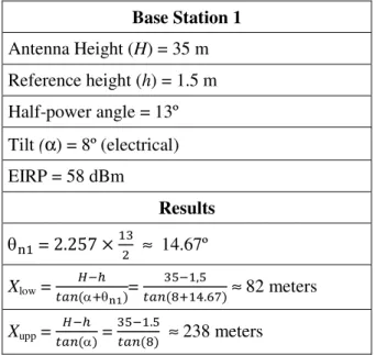
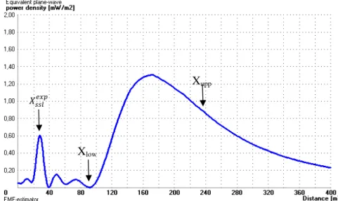
Table I presents some parameters of a typical base station and results applying equations (1b) and (2). Neglecting signal spread due to reflections (ground, buildings, trees etc), the maximum exposure will occur between 82 meters and 238 meters. Using the softwareEMF-Estimator, which is part of ITU-T Recommendation K.70 [5], it is shown in Figure 4 that the maximum exposure will occur approximately in 172 meters.
The software EMF-Estimator implements the point-source model and contains a library of the radiation patterns of transmitting antennas for a wide range of radiocommunication services. The point-source model is valid in the far field region, in the near-field region the results may overestimate or underestimate real levels [5]. As this software supports the application of ITU-T Recommendation K.70, it has a conservative view, where reflections may be considered, but always in a constructive, in-phase way with the direct signal. So, the results are the same of a free-space condition multiplied by a (1 + |Γ|)2 factor for power density calculations, where |Γ| is the absolute value of the surface reflection coefficient. In this software |Γ| can be set as 0 or 0.6. The accuracy of the results using this software is demonstrated in [2] comparing real measurements and in [5] presenting simulations where the values obtained with this software are compared with values obtained with the commercial software FEKO, that implements the Method of Moments.
Equations (1a), (1b) and (2) provides a rough estimation of the region where the maximum exposure may occur, taking into account only the main lobe. It is necessary to improve the estimation accuracy in order to have a useful tool.
TABLE I–TYPICAL BASE STATION PARAMETERS.
Base Station 1
Antenna Height (H) = 35 m Reference height (h) = 1.5 m Half-power angle = 13º
Tilt (α) = 8º (electrical) EIRP = 58 dBm
Results
= 2.257 × " ≈ 14.67º
Xlow = ( )=
"# ,#
(% &.'()≈ 82 meters
Xupp = ( ) =
"# .#
Figure 4 – Simulation using software EMF-Estimator. The point “illuminated” by the first null is easily identified in this graph, (Xlow). It is also clear that the maximum exposure will not occur in the point “illuminated” by the maximum emission (Xupp), but there are local peaks due to side lobes that depending on antenna characteristics
and tilt angle, could be responsible for a maximum exposure closer to the antenna mast ()**+,-.).
III. MATHEMATICAL FORMULATION
From Figure 4, it can be seen that just after Xlow,
/0
/ > 0, that is, the rate at which the power density changes with respect to the change in distance x is positive until reaching a maximum value, and //0 < 0 in the point Xupp. So, the objective is to find the point X, where /0/ = 0, subject to Xlow < X < Xupp. For a conservative estimation, the received power density in a two ray model is given by [13]:
1(2, 3, ∅) =5.6 .78(9,∅): ; ;8(9<,∅<):=> ?
&.@ Where:
1(2, 3, ∅) is the power density;
P is the power supplied to the antenna;
Gmax is the maximum gain of the antenna;
A(3, ∅) is the relative field pattern of the antenna;
A(3′, ∅′) is the relative field pattern of the antenna for the reflected signal;
|Γ| is the modulus of the reflection coefficient taking into account the wave reflected by the ground;
R is the distance between antenna and reference point;
R’ is the distance between the image of the antenna and reference point.
Considering reference points near ground level, the values of primed parameters can be approximated to the values of unprimed parameters, so that, considering a conservative view, the power density can be evaluated as [13]:
1(2, 3, ∅) =( ; ;)?.5.6&[email protected]2 .C(9,∅) (4)
Xlow
Xupp
DD
Where:
E(3, ∅) is the relative numerical gain and is numerically equal to FA(3, ∅)G .
Considering for this demonstration that the maximum exposure occurs in the direction of azimuth, that is, function E(3, ∅) can be considered as E(3). The main lobe of E(3) will be approximated by the normalized function cosq(θ), or in a general manner to include tilt, cosq(θ-α). This approximation is essential to have an analytical solvable derivative and is used as a model reference in [14] [15]. Following ITU-T Recommendation K.52 [13], the side lobe envelope will be approximated by a constant envelope Asl, given by the side lobe level (SLL), modulated by a short dipole factor (cos2θ). In the proposed model, parameter q is calculated considering the half-power angle !, as follows:
(5a)
E H I = 0.5 = KLMNH I, for main lobe and α = 0 (5b)
P = logT U log VKLM H !
2 IW
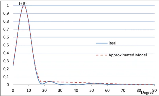
Figures 5 and 6 show the comparison of the proposed approximation with real antenna pattern, where the data sheet files were provided by manufacturers and Operators. The real antenna in Figure 5 has half-power angle of 10º, resulting q = 181.8062, and has electric tilt 7º. The real antenna in Figure 6 has half-power angle of 7º, resulting q = 371.2738, and has electric tilt 8º.
Considering the results for main lobe shown in Figure 5, the deviation of proposed approach from the real antenna until the half-power angle is less than 2%, and until the relative gain of -6 dB (0.25 in linear scale) is less than 7%. Using linear extrapolation it can be shown that at the relative gain of -9dB (0.125 in linear scale) has a 24% deviation or approximately 1 dB deviation, which means that while in the real pattern the gain is 9 dB below the maximum gain, in the approximated model, this value is 8 dB below.
Regarding TBXLHA-6565C-VTM antenna in Figure 6, it is informed by the manufacturer that the 3-dB angle is 7º (q = 371.2738). However, as data sheet is provided with gain information in every 1 degree, using linear extrapolation for a more accurate approximation, the 3-dB angle can be evaluated as 6.6836º (q = 407.2803). This represents a deviation of 6% for the relative gain of -6 dB and less than 1 dB deviation for the relative gain of -9 dB.
The same evaluation was done to Decibel Products - DB844H65T6EXY antenna resulting in equivalent results, i.e., less than 10% deviation for relative gain of -6 dB and less than 1 dB deviation for the relative gain of -9 dB.
For the tested antennas, the cosq(θ) model presented an excellent accuracy inside the half-power angle, a lightly overestimation inside the -6 dB angle and an acceptable overestimation inside the -9 dB angle (less than 1 dB deviation).
Most values of the side lobes envelope are higher than the real radiation pattern for the tested antennas. So, in a general manner, this model overestimates the exposure to EMF, except in some peak side lobes. For a conservative approach, a constant envelope equals to the side lobe level can be used.
(5c)
E(3) = X KLMN(3 − )
Z
M[. KLM (3 − ) \main lobe
Figure 5 – Comparison of Kathrein 742 265 antenna, with electrical tilt of 7º, with cosq(θ- ) model and side lobes envelope.
Figure 6 – Comparison of Andrews TBXLHA-6565C-VTM antenna, with electrical tilt of 8º, with cosq(θ- ) model and side lobes envelope.
Back to the proposed approach, applying main lobe eq. (5a) on eq. (4), and using the Pythagorean Theorem to replace R:
1(2, 3, ∅) =( ; ;)&[email protected]?.5.62 ( .] D)2^G(9 _) (6)
Recalling trigonometry that:
KLMN(3 − `) = (KLM3. KLM` + Mbc3. Mbc`)N (7)
0 0,1 0,2 0,3 0,4 0,5 0,6 0,7 0,8 0,9 1
0 10 20 30 40 50 60 70 80 90
Real
Approximated Model
0 0,1 0,2 0,3 0,4 0,5 0,6 0,7 0,8 0,9 1
0 10 20 30 40 50 60 70 80 90
Real
Approximated Model
F(θ)
Degree
And, accordingly Figure 1:
KLM3 =d ? ( )?OOO (8)
OOOMbc3 =d ? ( )?OOOOOO (9)
Applying equations (7), (8) and (9) in eq. (6), finding the derivative and equaling to zero:
e1 ef=
g h h h
i( ; ;)?.5.6 .j k
lk?m(nop)?.] D_
nop
lk?m(nop)?.Dq _r ^
&.@.[ 2 ( )2]
s t t t u<
= 0OOOOOO (10)
f = =l7( ). _.( ^?)> ?
.N.( )? ( ). _.( ^
?) (11)
Equations (11) and (5c) can be used to estimate the probable location of maximum exposure to EMF associated with a radio station. These equations prove that coincides with Xupp, only if the antenna is pointed directly to the floor. In other words, the angle of maximum radiation is not responsible for the maximum exposure point, except for = 90º.
In fact, the estimated value vwfxfy means that there is a local maximum exposure in a region containing this point. Scattered fields may shift the real local maximum exposure for a position closer to or farther from the radiocommunication station.
Nevertheless, it is possible to find real cases where side lobes causes higher exposure closer to the antenna than the main beam at a longer distance from the antenna. In order to provide guidance on how to predict from the antenna characteristics and tilt angle which gives higher exposure, equation (11) may be applied for side lobe, considering q = 2, in order to find X{{|}~•.
The result for q = 2 at distance X{{|}~• is an indication if the maximum exposure is due to side lobes, not necessarily the peak value is located at DD nor there is a huge confidence the main beam is not responsible for maximum exposure, once the envelope assumption overestimate almost all side lobes region. The accuracy of this side lobe envelope increases for antennas that have smaller side lobes levels at higher angles [13].
If power density calculated at X{{|}~• is higher than the evaluation at X€•‚}~• , then there is an indication that the side lobe may be responsible for the maximum exposure, otherwise there is an indication that the main lobe is responsible for the maximum exposure.
IV. TESTING THE PROPOSED APPROACH IN REAL AND SIMULATED SCENARIOS
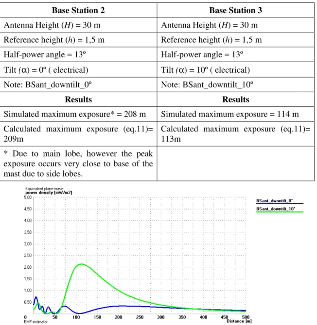
TABLE II–PARAMETERS OF BASE STATIONS 2 AND 3.
Base Station 2
Base Station 3
Antenna Height (
H
) = 30 m
Antenna Height (
H
) = 30 m
Reference height (
h
) = 1,5 m
Reference height (
h
) = 1,5 m
Half-power angle = 13º
Half-power angle = 13º
Tilt
(
α
) = 0º ( electrical)
Tilt
(
α
) = 10º ( electrical)
Note: BSant_downtilt_0º
Note: BSant_downtilt_10º
Results
Results
Simulated maximum exposure* = 208 m
Simulated maximum exposure = 114 m
Calculated maximum exposure (eq.11)=
209m
Calculated maximum exposure (eq.11)=
113m
* Due to main lobe, however the peak
exposure occurs very close to base of the
mast due to side lobes.
Figure 7 – Comparison of different electrical tilts for the same antenna. Results for Table II, considering base station 2 in blue line and for base station 3 in green line. For a scenario
with downtilt = 0º side lobe was responsible for the maximum exposure.
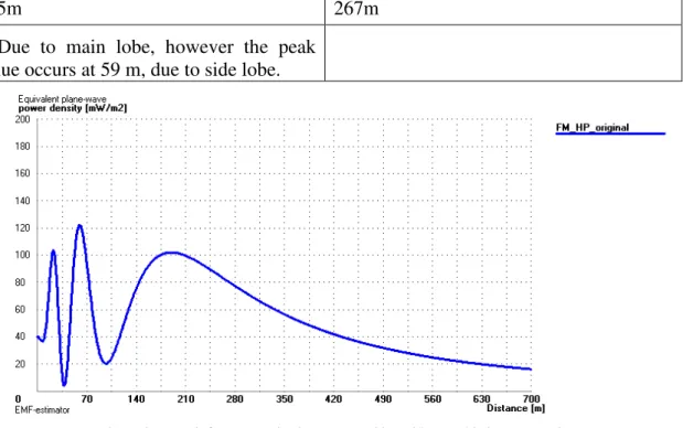
TABLE III–PARAMETERS OF A FMSTATION AND BASE STATION 4.
FM Station
Base Station 4
Antenna Height (
H
) = 37 m
Antenna Height (
H
) = 25 m
Reference height (
h
) = 1,5 m
Reference height (
h
) = 1,5 m
Half-power angle = 16,46º
Half-power angle = 7,5º (G = 18 dBi)
Tilt
(
α
) = 2,05º (electrical)
Tilt
(
α
) = 1º (mechanical)
Results
Results
Simulated maximum exposure * = 189 m
Simulated maximum exposure = 277 m
185m
267m
* Due to main lobe, however the peak
value occurs at 59 m, due to side lobe.
Figure 8 – Result for the FM Station presented in Table III. This is an example where side lobe is responsible of maximum exposure.
Figure 9– Result for the base station antenna with a lower half-power angle in the vertical plane (higher gain) given in Table III. The maximum exposure due to main lobe and sibe lobe are very close.
Figure 10 – Site located in the parking lot of “Mané Garrincha” stadium in Brasilia, Brazil. It is a co-located mast with 3 operators.
TABLE V–PARAMETERS OF REAL STATIONS
Operator 1 Operator 2
Antenna Height (H) = 37,4 m Antenna Height (H) = 25 m
Antenna Model: Andrew - TBXLHA-6565C-VTM
Antenna Model: Decibel Products - DB844H65T6EXY
Theoretical Diagram Set at 1920 MHz Theoretical Diagram Set at 880 MHz
Gain = 17.14 dBi Gain = 15.15 dBi
Mechanical Tilt (φ) = 0º Mechanical Tilt (φ) = 7º
Electrical Tilt (φ) = 8º Electrical Tilt (φ) = 6º
Antenna Vertical 3-dB bandwidth = 7º Antenna Vertical 3-dB bandwidth = 15º ± 1º
Antenna Polarization: Cross (45º) Antenna Polarization: Vertical
BCCH Frequency = 1875.8 MHz iDEN Control Channel = 857.2625 MHz
Measurement height (h) = 1.7 m Measurement height (h) = 1.7 m
Note: Coordinate Lat. 15° 46' 56.9'' Long. 47° 53' 44.4'' / Azimuth Measurement: 120°
Results
Results
Simulated maximum exposure = 203 m
Simulated maximum exposure = 72 m
Calculated maximum exposure (eq.11)=
207m
Calculated maximum exposure (eq.11)= 74
m
Measured maximum exposure = 30 m*
* due to local peak side lobe, however the
tendency shows that the maximum is
beyond 150 meters, as expected.
highest measure is at point 70 meters, as
expected.
The basic setup used for the tests was as follows:
- R&S TS-EMF (FSH Spectrum Analyzer, isotropic three-axis probe and laptop);
- Resolution bandwidth of 200 kHz for GSM signals and 30 kHz for iDEN signals;
- RMS Detector;
- Tripods with isotropic three-axis probe at 1.70 meter;
- Isotropic three-axis probe handle in a right angle in relation to the ground;
- 50-metres measuring tape;
- GPS;
- One measure per point, with time averaging;
- Surveyor’s body was not in the direct line of signal propagation and at least 2 meters away from the probe during measurements in order to mitigate the influence of body reflections.
The main characteristics of the R&S TS-EMF are:
- Frequency range: 30 MHz – 3 GHz;
- Measurement range: 1 mV/m – 100 V/m;
- Measurement uncertainty for electric field strength (confidence level 95%):
o ± 2.5 dB @ 0.9 GHz;
o ± 2.97 dB @ 1.8 GHz;
o ± 3.29 dB > 2.4 GHz.
This measurement equipment measures the E-field intensity in three orthogonal axes, where the spectrum analyzer switches sequentially each axis of the probe to get the combined E-field intensity.
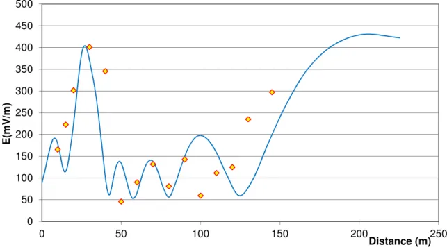
Figures 11 and 12 present the results of the evaluation of Operator 1 (GSM System) and Operator 2 (iDEN System) base stations. The measured values follow the estimated values, mainly for Operator 2 that has installed an antenna with few side lobes. The deviation of measured and estimated values is expected to be mainly due to reflections that are not taken into account in the simulations.
Considering a two-ray approach, the reflected signal can contribute with a constructive or a destructive way, depending on whether it arrives in-phase or out-of-phase with the direct signal. For a smaller wavelength (higher frequency) the variation of in-phase and out-phase contribution is faster along the radial being assessed. It should be considered as an error source the fact that theoretical antennas and real antennas might have different radiating pattern once installation cause perturbation in the antenna diagram, difference in the operating frequency and, also, side lobes nulls, depth and gains might also be a bit different.
Figure 11 presents the graph for a GSM system. The measurements show the oscillating behavior of side lobes and tendency of increasing signal due to main lobe. However, further measurements were not possible due to safety constraints, once after 145 meters busy streets occurred. So, the maximum exposure may occur on streets where the general public does not stay static. Applying equations (11) and (5c) the maximum exposure is expected to occur at 207 meters.
the main lobe, but this off-curve point is probably due to a constructive interference of the reflected signal. The second highest value is at point 70 meters, very close to the expected maximum exposure location, which is 74 meters.
Both simulations presented in Figures 11 and 12 were performed considering technical information available in the licenses for operation of the radiocommunication stations issued by the Regulatory Agency, complemented by Operators’ technical staff.
Figure 11 - Graph for the GSM system. The yellow dots represent the measured values, while the blue line represents the estimated values. It was not possible to measure at distances higher than 145 metres, once there were streets.
Figure 12 - Graph for a trunking (iDEN) system. The yellow dots represent the measured values, while the red line represents the estimated values. The peak value at 100 m is, probably, due constructive ray reflection.
0 50 100 150 200 250 300 350 400 450 500
0 50 100 150 200 250
E
(m
V
/m
)
Distance (m)
0 100 200 300 400 500 600 700 800 900 1000
0 50 100 150 200
E
(m
V
/m
)
V. UNCERTAINTY ANALYSIS
Using the proposed mathematical formulation is possible to estimate the local maximum exposure region associated with a radiocommunication station due to the main lobe. The case that showed the highest deviation was the first example, Base Station 1, see Table I and Figure 4. In that case, the calculations suggested that the maximum exposure occurs at about 182 meters, but the simulation identified as about 172 meters. In fact, considering that in both situations the reflection effect is being neglect, both results are, in practice, estimation.
Thus, for this example that resulted in the largest deviation, the difference between the calculations with equations (11) and (5c) represents a deviation of 5.8% for maximum exposure distance (182 meters versus 172 meters). However, the difference in power density between those two points is only 3.7% calculated in the simulation, while the difference in angle θ in which this maximum occurs is only 0.6 degrees (11.02° for the real antenna against 10.42º for the antenna model).
It is necessary to take into account the influence of the scattered signal in determining the maximum exposure point. The calculated point has to be considered as reference location, that the surveyor will consider as a center point in a region and look for signal intensity gradients to find the exact point of maximum exposure.
The proposed mathematical formulation was not exhaustively tested, but comparison results showed a good accuracy, mainly when is considered that reflection is a relevant phenomena, there is disturbance in the radiating diagram due to the installation locations, that the antenna data in simulation tools have an one-degree accuracy, and the installation data has an acceptable deviation established in regulation.
Considering |Γ| = 0.6 (conservative perspective), the real peak E-field intensity due to the main lobe is expect to be equal or less than 1.6 of the calculated E-field intensity peak neglecting reflections, however
continues to be the
reference point for a whole body EMF exposure evaluation. Instead of E-field intensity, it can be considered power density, S, replacing 1.6 by 2.56.The two real base stations evaluations results are consistent with the proposed methodology, as well as the five simulated scenarios.
VI. CONCLUSIONS
This paper presented a methodology to estimate the probable location of maximum exposure to EMF associated with a radiocommunication station, by applying an analytical expression, which takes into account information of height, vertical half-power angle and tilt of the antenna. Several simulations and comparisons were presented, and the largest deviation identified between simulation results and analytical expression results was 10 meters (182 and 172 m), representing less than 6%.
This methodology was also applied in real cases scenarios, showing consistent results. Calculated point must be considered as reference location, where surveyor will look for signal intensity gradients to find the exact point of maximum exposure, once scattered fields influence the maximum exposure location.
It was proven that the angle of maximum radiation is not responsible for the maximum exposure point, except when the antenna is pointed directly to the floor (tilt = 90º).
The proposed mathematical formulation is an important tool for assessing human exposure to EMF because the selection of measurement points is commonly visual and subjective, without taking into account the radiation diagram and characteristics of installation. In those common situations, what is being evaluated is the compliance of the measurement point, not the electromagnetic environment in the vicinity of the radiocommunication station, once the selected points might not represent the maximum exposure locations.
Thus, the results identified in this study are very important for those who evaluate the compliance of radiocommunication stations in relation to EMF exposure limits, as it presents an original and practical formulation, and the parameters required to perform the estimation of maximum exposure are included in radiocommunication station license and antenna datasheet.
ACKNOWLEDGMENT
The authors thank the Regional Office (UO01) and the Spectrum Management Division of Anatel (National Telecommunication Agency) for supporting the measurements in this work.
References:
[1] World Health Organization - Framework for developing health-based EMF standards. Available at http://www.who.int/peh-emf/standards/framework/en/
[2] Lewicki, F. ITU-T Technical Session on EMF – Comparison between measurement and calculations – EMF-Estimator, K.guide. Geneva, 27 May 2009, Available at
http://www.itu.int/ITU-T/worksem/techsessions/com05/090527/index.html
[3] IEC Standard 62232 - Determination of RF field strength and SAR in the vicinity of radiocommunication base stations for the purpose of evaluating human exposure.
[4] ITU-T Recommendation K-91 - Guidance for assessment, evaluation and monitoring of human exposure to radio frequency electromagnetic fields
[5] ITU-T Recommendation K-70 - Mitigation techniques to limit human exposure to EMFs in the vicinity of radiocommunication stations.
[6] ANATEL – Agência Nacional de Telecomunicações, "Resolução nº.303/2002 - Regulamento sobre Limitação da Exposição a Campos Elétricos, Magnéticos e Eletromagnéticos na Faixa de Radiofrequências entre 9 kHz e 300 GHz". ANATEL, 2002.
[7] A. Goldsmith, Wireless Communications, Cambridge University Press, 2005.
[8] Health Protection Agency (HPA) - Mobile Telephony and Health - Exposures from Base Stations.Available at http://www.hpa.org.uk/Topics/Radiation/UnderstandingRadiation/UnderstandingRadiationTopics/Electromagnetic Fields/MobilePhones/info_BaseStations/
[9] Terada, M. A. B. and Wanderley, P.H. Assessment of the influence of real-world radio station antennas. Brazilian Journal of Biomedical Engineering,Vol. 27 (Supp.1), p.45-51, Dec.2011.
[10] P.H. Wanderley & M.A. Terada (2012): Assessment of the applicability of the Ikegami propagation model in modern wireless communication scenarios, Journal of Electromagnetic Waves and Applications, 26:11-12, 1483-1491.
[11] Terada, M. A. Analysis of Electric Field Intensity of Radio Base Stations. Telecommunications Magazine (Inatel), vol. 11, nr. 01, May 2008 (in Portuguese).
[12] ITU-T Recommendation K-61 - Guidance to measurement and numerical prediction of electromagnetic fields for compliance with human exposure limits for telecommunication installations.
[13] ITU-T Recommendation K-52 - Guidance on complying with limits for human exposure to electromagnetic fields.
[14] C. A. Balanis, Antenna Theory: Analysis and Design, John Wiley & Sons, Inc., 2nd edition, pp. 48-53.