Abstract— The system resulting from the coupled Finite Element Method and Boundary Element Method formulations inherits all characteristics of both finite element and boundary element equation system, i. e., the system is partially sparse and symmetric and partially full and nonsymmetric. Consequently, to solve the resulting coupled equation system is not a trivial task. This paper proposes a new efficient lifting-based two level preconditioner for the coupled global system. The proposed approach is applied to solve the coupled systems resulting from the electromagnetic scattering problem and its performance is evaluated based on the number of iterations and the computational time. Traditional methods based on incomplete and complete LU decompositions are used for comparison.
Index Terms— FEM-BEM Equations, Lifting Technique, Preconditioner.
I- INTRODUCTION
THE FINITE ELEMENT and the Boundary Element Methods can be considered complementary to
each other in many cases. It is particularly true to problems where the domain considered is formed by
two (or more) regions where one of them is characterized by non-homogeneous material while the
other is free space. This kind of problem is difficult to be solved by any individual method described
above. Therefore, a combination of the two previous techniques comes up as a powerful way to solve
it [1].
The system resulting from the coupled Finite Element Method and Boundary Element Method
(FEM–BEM) formulations inherits all characteristics of both finite element and boundary element
equation system, i. e., the system is partially sparse and symmetric and partially full and
nonsymmetric [1], [2]. Consequently, the efficient solution of the FEM-BEM system has been object
of many researches [3], [4]. In fact, most of the proposed approaches are based on some adaptations.
In the algebraic multigrid context, for example, one should consider a fast matrix-by-vector
multiplication for dense matrices and to use some matrix approximation technique for the BEM dense
matrix. In particular, common smoother types do not work properly in the case of the single layer
potential [5]. In face of that, this work proposes a new efficient two level preconditioner for the global
An Efficient Two-Level Preconditioner
based on Lifting for FEM-BEM Equations
Fabio Henrique Pereira
Industrial Engineering Post Graduation Program – UNINOVE University-São Paulo, Brazil Marcio Matias Afonso
Electrical Engineering Department - Federal Technology Education Center - CEFET-Minas Gerais, Brazil João Antônio de Vasconcelos
Electrical Engineering Department – UFMG - Minas Gerais, Brazil Silvio Ikuyo Nabeta
FEM-BEM system based on the lifting technique [13]. This proposed approach is applied to some
real-life FEM-BEM coupled systems and its performance is evaluated based on the number of
iterations and the computational time. Traditional methods based on incomplete and complete LU
decompositions are used for comparison.
II.PROBLEM FORMULATION
The scattering problem was chosen to show the performance of the proposed approach. This kind of
problem occurs when an object is struck by an electromagnetic wave. To solve this problem by hybrid
technique an artificial surface must be chosen, which allows dividing scattering problems in two
regions. The first, Ω∞, is the free space with permeability µ0 and permittivity ε0. The second region
Ω may consist in general of non-homogeneous material with permeability µ(x,y) and permittivity )
, (x y
ε . Once the two regions are known, the electromagnetic fields in each one can be formulated.
These formulations for both interior and exterior fields can be then coupled at the boundary surface
through continuity conditions [1],[2],[6]. In this work, the formulation for both TMz and TEz
polarization are provided, the ejwt time convention is assumed and, the incident field uiZ( , )x y is given by
) sin cos
(
0 x s i y i
jk i
z e
u = ϕ + ϕ , (1)
Fig. 1. Dielectric cylinder illuminated by a
TM
z plane wave [2]A. Finite element formulation
The Helmholtz differential equation describes the field behavior in region Ω. In general form, the
Helmholtz equation could be written as [1]
(
1∇)
+ 02 2 =0⋅
∇ α u k α u , (2)
where, k0 =w µ0ε0 represents the wave number. Also, for electric field polarization α1=1/µr,
r ε
The strongproblem formulation for this case can be
expressed as it follows
: given α1, α2 and k0,find u such that [1]:
(
1∇)
+ 02 2 =0⋅
∇ α u k α u , ∀ x∈Ω (3)
ψ
α =−
∂ ∂
n u
1 ∀ x∈Γe (4)
φ =
u , ∀ x∈Γg (5) In above equations x=(x,y), Γe and Γg are exterior and Dirichlet boundary, respectively. Also, ψ
is the normal derivative and φ is the Dirichlet potential.
The weak formulation given by (6) is well known and its development will be omitted here [2].
(
)
∫ ∫∫Ω Ω Γ Γ=
∂ ∂ − Ω ⋅ − Ω ∇ ⋅
∇ 1 02 2 1 d 0
n u w d u w k d u
w α α α (6)
in which u is an approximation for the field and w is the weight function. The finite element
formulation given by (6) is computed in the target domain
and it is well suited to deal with
complex geometries
and anisotropic or isotropic
materials [2].Applying Galerkin’s procedure with (6) and dividing the domain in a grid of triangular elements, it
is possible to determine the general set of equations that can be written in matrix form as [2],
[ ]
K{ }
d +[ ]
C{ }
k =0 (7)where
[ ]
K is a n×n square matrix and[ ]
C is a n×m rectangular matrix, with m and n representing the total number of the nodes on the boundary and in the interior domain, respectively. Also,{ }
d is acolumn vector for approximated field arguments u and
{ }
k is a column vector for the normalderivative field arguments.
B. Boundary element formulation
In free space, Ω∞, the fields also are formulated by Helmholtz equation. The general formulation
for both electric and magnetic fields is:
) ( ) ( ) ( 02
2u r +k u r = f r
∇ , ∀r∈Ω∞ (8)
in which, for electric polarization u=Ez, f(r)= jk0Z0Jz−∇×Mi and for magnetic polarization z
H
u= , f(r)= j(k0 Z0)Mi−∇×Jz. Where, Z0 is the intrinsic impedance of the free space, Jz
represents all currents that flow along z-axis and Mi is the impressed magnetic source.
To formulate the fields in
Ω
∞, one introduces the free space Green’s function G0, which satisfies the differential equation) ' , ( ) ' , ( ) ' ,
( 02 0
0 2 r r r r G k r r
G + =−δ
and the Sommerfeld radiation condition [2]. In Eq. (9), δ
(
r−r')
represents the Dirac delta function. The solution for this equation is [2]( )
−= 02 0 '
' 0
4 1
, H k r r
j r r
G . (10)
The boundary fields are derived from the product of Eq. (8) by G0, the application of second scalar Green’s theorem and Dirac properties [1],[2].
' ' ' ' 0 ' ' ' 0 ' ( ) ) , ( ) , ( ) ( ) ( ) ( 5 .
0 Γ
∂ ∂ − Γ ∂ ∂ + =
⋅ ∫Γ ∫Γ d
n r u r r G d n r r G r u r u r
u i (11)
In Eq. (11), the primed sign indicates operation under integration point, the factor 0.5 is the solid
angle saw by the observer on the boundary and ui(r) is the incident field given by (1). Then, writing Eq. (11) for all m nodes on the boundary, it produces [1],[2]
{ } { }
u = b +[ ]
H{ }
d +[ ]
Q{ }
k , (12)in which,
[ ]
H and[ ]
Q are m×m matrices obtained from the discretization and{ }
b is a m×1 incident field column vector.C. Fem-Bem formulations
A typical finite element – boundary element system consists of two sets of equations, where
one of them is obtained from FEM (7) and other obtained on the boundary from BEM (12). As
the unknowns in both equations are the same, the two sets of equations could be coupled and
expressed in the in following form:
= − − = b k d Q H C K
Ax 0 (13)
This equation system inherits all characteristics of both finite element and boundary element
methods. For this reason, the equation system given by (13) is partially sparse and symmetric and
partially full and nonsymmetric [1]. There are many different ways to write FEM–BEM equation,
however the form present here is the easiest one [2]. The system is composed by N×N algebraic equations, N = (m + n), and solves both finite element and boundary element equation systems simultaneously. Although (13) is considered the best form to understand the coupled FEM–BEM
method it is not the better way to solve it because the symmetry of the FEM subsystem is not
exploited [2]. To write this system more efficiently see [2], [7]. Especial attention is required to
III-LIFTING BASED TWO-LEVEL PRECONDITIONER
The approach proposed here is based on a projection method. In this process an approximation for
the solution of the linear system (13) is extracted from a subspace of ℝNwhich is the search
subspace. If p is the dimension of , then the residual vector b−Ax is constrained to be orthogonal to the same subspace . Mathematically, denoting by V a N×p matrix whose column-vectors form a basis of , with an initial guess x0∈ , the approximate solution is written as
0
x=x +Vy, (14)
in which y is obtained solving the following system of equations from the orthogonality condition [8]
0
T T
V AVy=V r (15)
in which the initial residual vector is r0 = −b Ax0.
Then, if the p×p matrix V AVT is nonsingular, the expression for the approximate solution xɶ
becomes,
1
0 ( ) 0
T T
xɶ=x +V V AV −V r (16)
In the lifting based approach, the matrix V AVT is obtained by the decomposition of the matrix A
induced by the discrete lifting wavelet transform, with the wavelet of Haar [9].
The multiresolution analysis in discrete lifting wavelet transform decomposes the original grid
(space) Ω ∪ Ω∞ in two subspaces V and W such that 1
{ (2 )}k
V =span φ − x−k ∈ℤ (17)
1
{ (2 )}k
W=spanψ − x−k ∈ℤ (18)
and
V W
∞
Ω ∪ Ω = ⊕ (19)
where φ and ψ are the scaling and wavelets function, respectively, V is the low frequency and W the high frequency subspaces. The direct sum V⊕W in (19) means the sum of subspaces in which V and
W have only the zero vector in common [10].
Therefore, this approach can be viewed as a two-level multigrid algorithm in which VT is the restriction operator that represents a wavelet transform in equation form (lifting), as proposed in [11].
There are basically three forms for representing a wavelet transform: equation form (lifting),
filter form (filter bank) and matrix form. However, only the first two are appropriate in the
2 1 0
1 0
1 0
0 0 0 0
0 0 0 0 0 0
0 0 0 0
T N N h h h h V h h × = ⋯ ⋯ ⋯ ⋯ ⋮ ⋮ ⋮ ⋯ ⋯ ⋯
(20)
in which
= 2 1 , 2 1 ] ,
[h0 h1 are the low-pass filters coefficients associated to the haar wavelet. In this work, however, the application of the lifting restriction operator VT is algebraically
defined using the equation form of the wavelet transform as stated in (21), in which s
represents an approximation in the coarse grid of the original vector S, i. e., s = VTS.
1 2
For 1,..., /2 do [ ] [2 ] [2 1] [ ] [2 ] [ ] [ ] 2 [ ] End do
n N
d n S n S n
s n S n d n
s n s n
=
= − −
= +
=
(21)
The main advantages of this technique over the classical wavelet transform are:
a) Smaller memory requirement – the calculations can be performed in-place;
b) Efficiency: reduced number of floating point operations;
c) Parallelism –inherently parallel feature;
d) Easier to understand - not introduced using the Fourier transform;
e) Easier to implement;
f) The inverse transform is easier to perform – it has exactly the same complexity as the
forward transform;
g) Transforms signals with a finite length (without extension of the signal).
More details about these advantages as well as other important structural advantages of the
lifting can be found in [12], [13].
The computation of the coarse matrix V AVT is done applying the procedure (21) in the rows and columns of the original matrix A. If the number of rows and columns in matrix A is not
even, a zero padding operation is accomplished adding one sample with value zero at the end of
the rows and columns in order to achieve the desired length [12]. So, the resulting V AVT matrix will be formed by the detail coefficients obtained from the discrete lifting wavelet transform and
will represent an approximation in the coarse grid of the matrix A which is defined as (13).
The procedure defined in (21) represents the Haar transform in the lifting scheme. Haar is the
simplest possible wavelet and it is associated to shorter filters [12]. There are many other wavelet
functions that can present better approximation properties in many cases, but the choice for short
This two-level preconditioner is illustrated in Fig. 2 and it can be represented by the following
algorithm:
:
-: ,
: 1.
2.
T Algorithm two level lifting preconditioner
Input the right hand side vector b the original matrix A
and the coarse grid matrix V AV
Output approximation x
Choose an initial guess x
C
ɶ
1 3. ( ) 4.
5.
T T
ompute the residual vector r b Ax
e V AV V r
x x Ve
Return x
−
= −
= = +
ɶ
ɶ
As the matrix A is partially sparse and the procedure defined in (21) is the Haar transform, the resulting matrix will also be partially sparse and it can be created explicitly even for very large
problems. However, if an iterative method was used to solve the coarse grid system in line 3 of the
algorithm the matrix V AVT has not to be explicitly created.
Fig. 2. Two-level lifting preconditioner
IV-NUMERICAL RESULTS
The Lifting based two-level method (LTL) was applied as a preconditioner for the Stabilized
Bi-Conjugate Gradient Method (BiCGStab) in the solution of three global coupled FEM-BEM systems.
These systems were obtained for a circular cylinder with 0.3λ diameter, εr=3 and wave length λ=1. The cylinder is struck by a TMz plane wave with incident angle of θi =180o.
The results related to the number of iterations and setup and solver times are presented in tables I, II
and III. The number of iterations corresponds to the number of BiCGStab steps necessary to reduce
the Euclidean norm of the residual vector to the order of 10-4, which was considered enough to
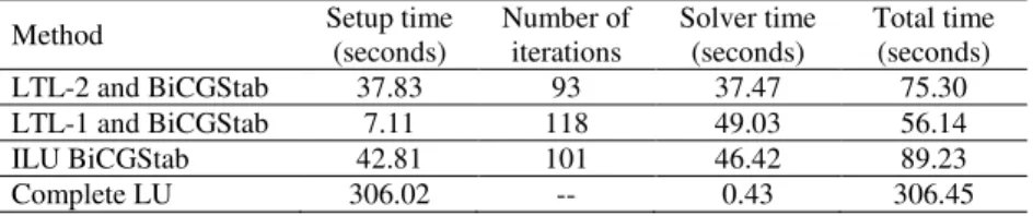
In Tables I to III, N and NZ stand for the number of rows and the number of nonzero entries in the matrix, respectively.
In the tests, the system with the V AVT matrix in LTL was solved by incomplete LU solver (LTL-1)
and with a direct method based on the complete LU decomposition (LTL-2). So, the setup time
presented includes the computation of a explicit representation of the coarse matrix V AVT . Such
representation of the coarse matrix has a sparsity pattern similar to the original matrix (Fig. 3) and it
can be created in a relative small computational time, as can be viewed in the setup time column from
tables I, II and III. The Incomplete LU (ILU) preconditioner and the complete LU solver were used
for comparison.
TABLEI:RESULTS FOR A SMALL GLOBAL FEM-BEM MATRIX (N=2119,NZ=87133)
Method Setup time
(seconds)
Number of iterations
Solver time (seconds)
Total time (seconds)
LTL-2 and BiCGStab 37.83 93 37.47 75.30
LTL-1 and BiCGStab 7.11 118 49.03 56.14
ILU BiCGStab 42.81 101 46.42 89.23
Complete LU 306.02 -- 0.43 306.45
TABLEII:RESULTS FOR A MEDIUM GLOBAL FEM-BEM MATRIX (N=3869,NZ=1073183)
Method Setup time
(seconds)
Number of iterations
Solver time (seconds)
Total time (seconds)
LTL-2 and BiCGStab 280.59 127 414.24 694.83
LTL-1 and BiCGStab 260.70 183 570.80 831.50
ILU BiCGStab 1358.05 151 1171.22 2529.27
Complete LU 2057.25 -- 6.11 2063.36
TABLEIII:RESULTS FOR A LARGE GLOBAL FEM-BEM MATRIX (N=10389,NZ=1148163)
Method Setup time
(seconds)
Number of iterations
Solver time (seconds)
Total time (seconds) LTL-2 and BiCGStab 3114.78 195 1259.8 4374.58 LTL-1 and BiCGStab 636.45 362 1679.03 2315.48
ILU BiCGStab 1587.41 327 1845.56 3432.97
Complete LU >10000.00 -- -- --
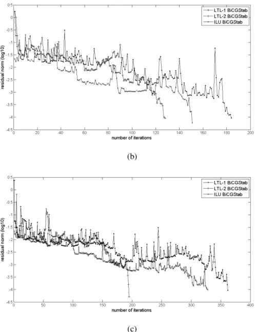
The convergence histories for the tests are illustrated in Fig. 4. The convergence history shows the
residual norm after the first preconditioner step what explains the difference in the start point
of the convergence curves. As the initial guess was the zero vector, the initial residual norm is
Fig. 3. Sparsity pattern for original (upper) and coarse approximation (bottom) matrices
(b)
(c)
Fig. 4. Convergence history for the small (a), medium (b) and large (c) problems.
CONCLUSIONS AND COMMENTS
The approach proposed in this work revealed to be very efficient and promising to solve the global
systems of coupled FEM-BEM equations, mainly for the medium and large problems. The usual
complete LU decomposition method is a good choice for small problems, but is very expensive for
larger problems, as can be viewed in Table II.
For large problems, where an efficient preconditioner is required, the lifting two-level method gives
the best results. In this case, the LU decomposition can be used to solve efficiently the coarse system
which has the half of unknowns (see Table III). Concerning the computational time the proposed
approach was about 80% faster than the classical ILU preconditioner. Also, regarding the
convergence rate, the numerical results suggest that the number of iterations necessary to reach a
given accuracy grows only logarithmically with the number of unknowns. Further tests have to be
About the coarse system solution (step 3 in the algorithm), the coarse matrix VTAV should be explicitly assembled if an incomplete or complete LU solver is used in this step. However, this is not
a problem since the resulting matrix is partially sparse as can be seen in Fig. 3, and it can be created
explicitly even for very large problems. Also, regarding the memory requested it can be seen that the
operator complexity of this preconditioner, which is defined as the sum of number of nonzero entries
in the coarse matrix and its ILU factors divided by the number of nonzero entries in the matrix A, is
something about 80% of operator complexity in the ILU preconditioner. It indicates the total storage
space required by the preconditioner matrices and it is generally considered a good indication of the
preconditioning operation cost in multigrid approaches.
One alternative is using an iterative solver such as BiCGStab, where it is enough to know the action
of the system matrix on a given vector, but the preconditioning of the coarse system is difficult to be
achieved
in this case
.Finally, it is important to say that the proposed method can be applied in different kind of linear
system, complex or real, symmetric or non-symmetric, sparse or dense matrices, and it can be a good
alternative in those cases in which the conventional block-diagonal preconditioning for Schur
complement based or hierarchical basis solvers do not produce good results.
ACKNOWLEDGMENT
The authors would like to thank FAPESP (2009/11082-2) and CNPq for the financial support.
REFERENCES
[1] M. M. Afonso, J. A. Vasconcelos, “Two dimensional scattering problems solved by finite element – boundary element method”, In: 22th CILAMCE - Iberian Latin-American Congress on Computational Methods in Engineering, 2001. [2] J. Jin, The finite element method in electromagnetics, Wiley, New York, 1993.
[3] G. Aiello, S. Alfonzetti, E. Dilettoso, N. Salerno, “An Iterative Solution to FEM-BEM Algebraic Systems for Open-Boundary Electrostatic Problems”, IEEE Trans. on Magnetics, vol. 43, n. 4, pp. 1249 – 1252, 2007.
[4] P. Mund and E. P. Stephan, “Adaptive Coupling and Fast Solution of FEM-BEM Equations for Parabolic-Elliptic Interface Problems”, Math. Methods in the Appl. Scienc., vol. 20, n. 5, pp. 403-423, 1998.
[5] D. Pusch, Efficient Algebraic Multigrid Preconditioners for Boundary Element Matrices, Phd thesis.Johannes Kepler University Linz, Austria, 1997.
[6] A. C. Balanis, Advanced engineering electromagnetics, Wiley, New York, 1989.
[7] N. Lu and J. M. Jin, “Application of fast multipole method to finite – element boundary – integral solution of scattering problems”, IEEE Transaction on antennas and propagation, vol. 44, n. 6, pp. 781 – 786, 1996.
[8] Y. Saad, Iterative Methods for Sparse Linear Systems, 2nd ed., SIAM, Philadelphia, 2003.
[9] T. K. Sarkar, S. P. Magdalena, C.W. Michael, Wavelet Applications in Engineering Electromagnetics, Artech House, Boston, 2002.
[10]K. H. Rosen, (Ed.). Handbook of Discrete and Combinatorial Mathematics. Boca Raton, FL: CRC Press, 2000, pp. 357. [11] F. H. Pereira and S. I. Nabeta, “Wavelet-Based Algebraic Multigrid Method Using the Lifting Technique”, Journal of
Microwaves, Optoelectronics and Electromagnetic Applications, vol. 9, n. 1, 1-9, 2010.
[12]A. Jensen, A. la Cour-Harbo, The Discrete Wavelet Transform, Ripples in Mathematics, Springer, Berlin 2001, pp. 21. [13]W. Sweldens. “The lifting scheme: A custom-design construction of biorthogonal wavelets”. Appl. Comput. Harmon.
![Fig. 1. Dielectric cylinder illuminated by a TM z plane wave [2]](https://thumb-eu.123doks.com/thumbv2/123dok_br/18887443.424152/2.892.108.780.439.902/fig-dielectric-cylinder-illuminated-tm-z-plane-wave.webp)