Spatio-temporal SNN : integrating time and space in the clustering process

(1)

Universidade do Minho

Escola de Engenharia

João Ricardo Leite Mota Oliveira

Spatio-temporal SNN: Integrating Time and

Space in the Clustering Process

UMinho|20 13 João Ricar do Leit e Mo ta Oliv eir a

Spatio-temporal SNN: Integrating Time and Space in t

he Clus

(2)

Dissertação de Mestrado

Mestrado em Engenharia e Gestão de Sistemas de Informação

Trabalho realizado sob orientação da

Professora Doutora Maribel Yasmina Santos

Universidade do Minho

Escola de Engenharia

João Ricardo Leite Mota Oliveira

Spatio-temporal SNN: Integrating Time and

Space in the Clustering Process

(3)

(4)

João Ricardo Leite Mota Oliveira Acknowledgments

ACKNOWLEDGMENTS

Although this work is individual, many people directly or indirectly contributed for its development. Without their help, the quality of this work would surely be inferior. To all of them I would like to express my appreciation, but cannot help showing my special gratitude:

Firstly, to my advisor, Professor Maribel Yasmina Santos, for sharing her knowledge and experience, for her countless theoretical and technical contributions to this work, for the given motivation in difficult times and for trusting me to complete this project.

To Professor João Moura-Pires for his opinions and text reviews. To Guilherme and Fernando, project colleagues, for the brainstorming meetings, and for helping me to familiarize with the tool used in this project.

To Sérgio, Joana and Rui, “brothers in arms” in this little adventure that was the master’s degree, for the constant exchange of ideas and the companionship in this lonely work.

To Adriano, Frederico and Gonçalo, long-time friends, for the social moments and relaxing times needed to distract the mind from work.

Finally, a very special thanks to my family, my father João Daniel and my mother Maria Salomé for the education and personal values passed on, making me the person I am today. For giving me all the necessary conditions so I could complete this degree, and for always believing in my abilities, even when I did not give them reason to. I would also like to thank my brother Tiago for all the moments of fun and joy throughout life.

This work was done with the support of the research project “GIAP - GeoInsight Analytics Platform (LISBOA-01-0202-FEDER- 024822)”, funded by Comissão de Coordenação e Desenvolvimento Regional de Lisboa e Vale do Tejo (PORLisboa), included in Sistema de Incentivos à Investigação e Desenvolvimento Tecnológico (SI I&DT), through the research fellowship UMINHO/BI/304/2012.

(5)

(6)

João Ricardo Leite Mota Oliveira Abstract

ABSTRACT

Spatio-temporal clustering is a new subfield of data mining that is increasingly gaining scientific attention due to the technical advances of location-based or environmental devices that register position, time and, in some cases, other semantic attributes. This process intends to group objects based in their spatial and temporal similarity helping to discover interesting patterns and correlations in large datasets. One of the main challenges of this area is that there are different types of spatio-temporal data and there is no general approach to treat all these types. Another challenge still unresolved is the ability to integrate several dimensions in the clustering process with a general-purpose approach. Moreover, it was also possible to verify that few works address their implementations under the SNN (Shared Nearest Neighbour) algorithm, which gives the opportunity to propose an innovative extension of this particular algorithm.

This work intends to implement in the SNN clustering algorithm the ability to deal with spatio-temporal data allowing the integration of space, time and one or more semantic attributes in the clustering process. In this document, background knowledge about clustering, spatial clustering and spatio-temporal clustering are presented along with a summary of the main approaches followed to cluster spatio-temporal data with different clustering algorithms. Based on those approaches, and in the analysis of their advantages and disadvantages, the boundaries of this work are defined in order to incorporate the space, time and semantic attribute dimensions in the SNN algorithm and thus propose the 4D+_{SNN approach.}

The results presented in this work are very promising as the approach proposed is able to identify interesting patterns on spatio-temporal data. Concretely, it can identify clusters taking into account simultaneously the spatial and temporal dimension and it also has good results when adding one or more semantic attributes.

Keywords: Clustering; Density-based Clustering; Spatio-temporal Data; Distance

(7)

(8)

João Ricardo Leite Mota Oliveira Resumo

RESUMO

O clustering espaço-temporal é uma nova área do data mining que está a ganhar crescente atenção por parte da comunidade científica devido aos avanços tecnológicos dos dispositivos de localização ou monitorização ambiental que registam posição, tempo e, em alguns casos, outros atributos semânticos. Este processo pretende agrupar objectos segundo as suas similaridades espaciais e temporais ajudando assim a descobrir padrões interessantes e correlações em grandes conjuntos de dados. Um dos grandes desafios nesta área é a existência de vários tipos de dados espaço-temporais e não existe uma abordagem geral para tratar todos estes tipos. Outro desafio ainda por resolver é a capacidade para integrar várias dimensões no processo de clustering com uma abordagem geral. Além disso, foi possível verificar que poucos trabalhos de investigação usam o algoritmo SNN (Shared Nearest Neighbour) nas suas implementações o que dá a oportunidade para propor uma extensão inovadora para este algoritmo em particular.

Este trabalho pretende implementar no algoritmo de clustering SNN a capacidade para lidar com dados espaço-temporais permitindo assim a integração do espaço, tempo e um ou mais atributos semânticos no processo de clustering. Neste documento, serão apresentados alguns conceitos sobre clustering, clustering espacial e clustering espaço-temporal assim como um resumo das principais abordagens usadas para fazer o clustering de dados espaço-temporais com algoritmos de clustering diferentes. Baseado nestas abordagens e na análise das suas vantagens e desvantagens, serão definidos os limites deste trabalho de modo a incorporar as dimensões espaço, tempo e atributo semântico no algoritmo SNN e, assim, propor a abordagem 4D+_SNN.

Os resultados apresentados neste trabalho são bastante promissores pois a abordagem proposta é capaz de identificar padrões interessantes em dados espaço-temporais. Concretamente, consegue identificar clusters tendo em consideração simultaneamente as dimensões espaço e tempo e também obtém bons resultados quando adicionando um ou mais atributos semânticos.

(9)

(10)

João Ricardo Leite Mota Oliveira Table of Contents

LIST OF FIGURES

Figure 1 - Design Science Research Process. ... 5

Figure 2 - Data Mining as a Step in the Knowledge Discovery Process. ... 8

Figure 3 - Clustering Results with Different Values of k. ... 14

Figure 4 - Map of London by John Snow. ... 16

Figure 5 - Example of Spatial Data. ... 16

Figure 6 - Monthly Precipitation in November 2006. ... 17

Figure 7 - Map of Altitudes of the Iberian Peninsula. ... 18

Figure 8 - Example of Geo-referenced Variables. ... 20

Figure 9 - Example of Moving Objects. ... 21

Figure 10 - Example of Geo-referenced Time Series. ... 22

Figure 11 - Example of Trajectories. ... 23

Figure 12 - Spatio-temporal Neighbourhood. ... 26

Figure 13 - The REMO Process. ... 27

Figure 14 - Classification of Movement Patterns. ... 28

Figure 15 - Dataset with an Overlapped Grid... 36

Figure 16 - Sample with the First Elements of the Differences List Divided by k Intervals. ... 37

Figure 17 - Sample with the Last Elements of the Differences List Divided by k Intervals. ... 39

Figure 18 - Sorted 3-dist Graph. ... 39

Figure 19 - Result of the Valleys Approach for the Temporal Dimension for t5.8k.a Dataset. ... 40

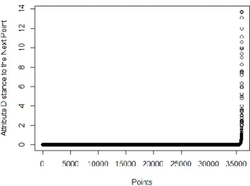
Figure 20 - Sorted Distances in t5.8k. ... 41

(13)

List of Figures João Ricardo Leite Mota Oliveira

Figure 22 - Sorted Temporal Distances in t5.8k.a. ... 43

Figure 23 - Sorted Attribute Distances in Fires 2011 Dataset. ... 44

Figure 24 - Spatial Deciles Result for t5.8k. ... 44

Figure 25 - Temporal Deciles Result for t5.8k.a. ... 44

Figure 26 - Temporal Deciles Result for t5.8k.b. ... 44

Figure 27 - Attribute Decile Result for Fires 2011 Dataset. ... 45

Figure 28 - Spatial Distribution of t5.8k Dataset. ... 48

Figure 29 - Temporal Distribution of t5.8k.a. ... 49

Figure 30 - Temporal Distribution of t5.8k.b. ... 49

Figure 31 - Result of Spatio-temporal Clustering for t5.8k.a Using 50%-50% Weights (SNN Parameters, k = 40, Eps = 16, MinPts = 24). ... 50

Figure 32 - Result of Spatio-temporal Clustering for t5.8k.b Using 20%-80% Weights (SNN Parameters, k = 40, Eps = 16, MinPts = 24). ... 50

Figure 35 - Spatial Distribution of t4.8k. ... 51

Figure 36 - Result of Spatio-temporal Clustering Using 50%-50% Weights (SNN Parameters, k = 40, Eps = 16, MinPts = 24). ... 52

Figure 37 - Result of Spatio-temporal Clustering Using 75%-25% Weights (SNN Parameters, k = 40, Eps = 16, MinPts = 24). ... 52

Figure 38 - Spatial Distribution of the Fires 2011 Dataset. ... 53

Figure 39 - Clustering of the Fires 2011 Dataset Using 50%-50% Weights (SNN Parameters, k = 230, Eps = 45, MinPts = 200). ... 54

Figure 40 - Clustering of the Fires 2011 Dataset Using 50%-50% Weights (SNN Parameters, k = 230, Eps = 45, MinPts = 200) (Temporal Perspective). ... 55

(14)

João Ricardo Leite Mota Oliveira List of Figures

Figure 41 - Clustering of the Fires 2011 Dataset Using 33%-34%-33% Weights (SNN Parameters, k = 230, Eps = 45, MinPts = 200). ... 56 Figure 42 - Clustering of the Fires 2011 Dataset Using 33%-34%-33% Weights (SNN Parameters,

k = 230, Eps = 45, MinPts = 200) (Temporal Perspective)... 56 Figure 43 - Number of Points, Maximum and Minimum per Cluster (Same Weights for the 3

Dimensions). ... 57 Figure 44 - Clustering of the Fires 2011 Dataset Using 20%-20%-60% Weights (SNN Parameters,

k = 230, Eps = 45, MinPts = 200). ... 59 Figure 45 - Clustering of the Fires 2011 Dataset Using 20%-20%-60% Weights (SNN Parameters,

k = 230, Eps = 45, MinPts = 200) (Temporal Perspective)... 59 Figure 46 - Number of Points, Maximum and Minimum per Cluster Using 20%-20%-60% Weights. ... 60 Figure 47 - Clustering of the Fires 2012 Dataset Using 33%-34%-33% Weights (SNN Parameters,

k = 230, Eps = 45, MinPts = 200). ... 62 Figure 48 - Clustering of the Fires 2012 Dataset Using 33%-34%-33% Weights (SNN Parameters,

k = 230, Eps = 45, MinPts = 200) (Temporal Perspective)... 62 Figure 49 - Clustering of the Fires 2011-2012 Dataset Using 33%-34%-33% Weights (SNN

Parameters, k = 230, Eps = 45, MinPts = 200). ... 64 Figure 50 - Clustering of the Fires 2011-2012 Dataset Using 33%-34%-33% Weights (SNN

Parameters, k = 230, Eps = 45, MinPts = 200). ... 64 Figure 51 - Map of Portugal with the Meteorological Stations. ... 66 Figure 52 - Clustering of the Meteo1 Dataset Using 33%-34%-33% Weights (SNN Parameters, k =

50, Eps = 18, MinPts = 45). ... 67 Figure 53 - Clustering of the Meteo2 Dataset Using 25% Weight for the 4 Dimensions (SNN

Parameters, k = 50, Eps = 18, MinPts = 45). ... 68 Figure 54 - Example of Bounding Box Problem. ... 73

(15)

(16)

João Ricardo Leite Mota Oliveira List of Tables

LIST OF TABLES

Table 1 - Sample Dataset of Spatio-temporal Events. ... 20

Table 2 - Sample Dataset of Geo-referenced Time Series. ... 22

Table 3 - Sample Dataset of Trajectories. ... 23

Table 4 - Example of a Geo-referenced Dataset. ... 31

Table 5 - Number of Points and Statistics of the Burnt Area per Cluster in Fires 2011 Dataset (33%-34%-33% Weights). ... 58

Table 8 - Number of Points and Statistics of the Burnt Area per Cluster in Fires 2011-2012 Dataset (33%-34%-33% Weights). ... 65

Table 9 - Number of Points and Statistics of the Burnt Area per Cluster in Meteo1 Dataset (33%-34%-33% Weights). ... 67

Table 10 - Number of Points and Statistics of the Burnt Area per Cluster in Meteo2 Dataset (25%-25%-25%-25% Weights). ... 69

(17)

(18)

João Ricardo Leite Mota Oliveira List of Acronyms and Abbreviations

LIST OF ACRONYMS AND ABBREVIATIONS

BIRCH Balanced Iterative Reducing and Clustering using Hierarchies CLARA Clustering Large Applications

CLARANS Clustering Large Applications based on Randomized Search CLIQUE CLustering In QUEst

CURE Clustering Using REpresentatives

DBSCAN Density-Based Spatial Clustering of Applications with Noise DENCLUE DENsity-based CLUstEring

DSR Design Science Research GPS Global Positioning System

OPTICS Ordering Points to Identify the Clustering Structure PAM Partitioning Around Medoids

ROCK RObust Clustering using linKs SNN Shared Nearest Neighbour STING Statistical Information Grid

(19)

(20)

João Ricardo Leite Mota Oliveira Introduction

1 - INTRODUCTION

This chapter introduces the area of this work and the motivation for undertaking it. It will be demonstrated why this work is important and presented the research question. After that, the objectives outlined for this project and the expected results for this work are presented. Then, some considerations about the methodology used in this work are reported. In the end of this chapter is presented the structure of this report.

1.1 - Framework and Motivation

Nowadays, great amounts of data are being collected by organizations. Besides the progress in this collection, the analysis of these data for decision support is still a great challenge, as these organizations cannot know beforehand what information is useful for their business or not (Han, Kamber, & Pei, 2012).

When dealing with spatio-temporal data, in addition to these challenges, we must consider the complexity of handling the space in which the events occurred and the moment in time in which they were verified. This analysis of movement patterns in spatio-temporal data is a relatively new area of research and is becoming gradually more important because large amounts of spatio-temporal data are being generated by devices like cell phones, GPS (Global Positioning System) and remote sensor devices (Tork, 2012).

These data introduce new challenges to data analytics and require new techniques for knowledge discovery and spatio-temporal clustering can be one of these new techniques. This new sub field of Data Mining is gaining high popularity especially in geographic information sciences due to the availability of cheap sensor devices which caused an exponential growth of geo-tagged data in the last years. The great challenge is not to get the right data but to analyse all the data we can get (Kisilevich, Mansmann, Nanni, & Rinzivillo, 2010). One key aspect is that it is possible to analyse all these data because, only in the last years, the necessary technological development was achieved that enabled the discovery of knowledge in vast amounts of data (Laube, Wolle, & Gudmundsson, 2007).

(21)

Introduction João Ricardo Leite Mota Oliveira

The analysis of spatio-temporal data is very complex because it involves time, geographical space, objects appearing and disappearing in space and multidimensional attributes that are in constant change over time (Andrienko et al., 2011).

The usual clustering approaches do not consider time and space. The ones that consider can only process spatio-temporal events but cannot treat moving objects because this is a complex type of data (Birant & Kut, 2007; Liu, Deng, Bi, & Yang, 2012). Therefore, the discovery of spatio-temporal clusters is a challenging issue in the knowledge discovery domain and is very important in many areas of science and technology such as meteorology, biology, sociology, transportation engineering, telecommunications, etc. (Dodge, Weibel, & Lautenschütz, 2008). These techniques are used essentially to get patterns of animal behaviour, human movement and traffic, surveillance, security, military and even sports movement (Laube et al., 2007).

From all the families of clustering algorithms, the density-based seems to be a good candidate as it will be demonstrated in the next chapters. From the algorithms in the density-based family, the Shared Nearest Neighbour (SNN) algorithm seems to be an appropriate choice for this project as it will be demonstrated by some studies presented in the literature review.

The SNN algorithm is a density-based clustering algorithm that can identify clusters of different sizes, shapes and densities. Moreover, it can identify noise objects in the data (Ertoz, Steinbach, & Kumar, 2002). In order to measure the similarity between data objects, a distance function is necessary. The most common distance function is the Euclidean distance among objects. The choice of this function is very important because it influences greatly the resulting clusters (Lin, Xie, Song, & Wu, 2009). Some authors add the time dimension to this distance function in order to cluster spatio-temporal data transforming a 2D vector into a 3D vector of with x and y representing the spatial coordinates and t the time in which the position was recorded (Tork, 2012).

This all brings us to the research question: “How can we integrate the space and time dimensions in the clustering of spatio-temporal data using the SNN algorithm?” To answer this question, an extensive bibliography research was done to know what the main techniques that researchers are using in the spatio-temporal clustering area. With that knowledge, it was expected to implement a working prototype, following a defined approach, which can discover clusters in spatio-temporal datasets using the SNN algorithm.

(22)

This work is part of the project “Geo Insight Analytics Platform” leaded by Novabase Business Solutions, which intends to develop a platform that enables the analysis, correlation and visualisation of spatio-temporal data for the telecommunication business.

1.2 - Objectives and Expected Results

In order to answer the research question of this project: “How can we integrate the space and time dimensions in the clustering of spatio-temporal data using the SNN algorithm?” some objectives and expected results were defined.

Clustering spatio-temporal data implies the inclusion of space and time when looking for similarities. In order to be able to add these two dimensions to the clustering process, different distance functions that measure the similarity between objects need to be defined, implemented and tested. Besides the several distance functions, which allow the identification of different types of clusters, the granularity of space and time plays a major role in the clustering process. Along with the spatial and temporal dimension, it is necessary to understand how other dimensions can be added to the clustering process.

This work has as main goal the integration of space and time and one or more semantic attributes in the clustering process, allowing the temporal cataloguing of events and the verification of the clusters evolution across time.

For the accomplishment of this goal, several objectives were set:

 Identification of the several types of spatio-temporal data and their corresponding characteristics;

 Identification of the current approaches that cluster spatio-temporal data as well as their advantages and disadvantages;

 Conceptualization of an approach to cluster spatio-temporal data with or without semantic attributes;

 Implementation of a prototype that uses the SNN algorithm to cluster spatio-temporal data with or without semantic attributes following the proposed approach;

 Validation of the implemented prototype and verification of the quality of the obtained clusters.

(23)

Introduction João Ricardo Leite Mota Oliveira

The expected results are:

 An approach to cluster spatio-temporal data;

 A working prototype that can cluster spatio-temporal data;

 A sensibility analysis of the influence of each input parameter of the SNN algorithm in the proposed approach.

1.3 - Methodology Approach

So this project can run smoothly and without delays, several research methodologies were studied and Design Science Research (DSR) was chosen because it gives the principles, practices and procedures required to finish a work successfully in this area. This methodology is well known in the Information Systems area and it has been used with good results in several studies (Peffers, Tuunanen, Rothenberger, & Chatterjee, 2007).

Besides its applicability to the Information Systems area, DSR is appropriate to this work as it intends to build an artefact that solves a real problem helping in the development of the theory in this area (Hevner, March, Park, & Ram, 2004). Using this methodology, it is expected that the project runs more smoothly and faster than using an ad-hoc approach.

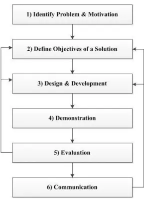
The DSR methodology involves six steps (Peffers et al., 2007): Problem Identification and Motivation, Definition of the Objectives for a Solution, Design and Development, Demonstration, Evaluation and, lastly, Communication.

The methodology is structured in a sequential order but the researcher does not have to do all steps in sequential way. Going back to a previous step may be needed to achieve better results at the end of this process. The methodology and all the connections between steps can be seen in Figure 1.

Applying this methodology to the project in hands, in the first step, it required a literature review in the spatio-temporal clustering area in order to acquire knowledge about the problem. It was also necessary to do a contextualization with the GeoInsight Analytics Platform project in order to understand what has already been done and what are the problems that need to be solved. In the next step, it was defined the objectives that the artefact should achieve according to the context of the problem.

(24)

Figure 1 - Design Science Research Process.

Then, the development phase began and a prototype that can be used to cluster spatio-temporal data was implemented.

After that, a long series of tests to the prototype were made. These tests involved the use of synthetic datasets as well as real datasets. The results of these tests were analysed in order to perceive the efficacy and efficiency of the prototype. If the results were not the expected ones for this solution, the prototype went back to the design step in order to improve the results and achieve the optimal solution to the problem.

Lastly, all the process and its contribution were published as a dissertation of a master thesis and as a publication of a paper in an international conference.

1.4 - Structure of the Report

This work is organized as follows. In Chapter 2 the main concepts of this work are described as well as the SNN algorithm. The current approaches used to cluster spatio-temporal data will also be presented. Chapter 3 describes the proposed approach, 4D+_{SNN, the types of}

used spatio-temporal data and the heuristics proposed in this work. Chapter 4 presents the obtained results clustering two synthetic datasets and three real datasets. Finally, Chapter 5 concludes this document with a summary of the main findings and proposals of future work.

(25)

(26)

João Ricardo Leite Mota Oliveira Conceptual Framework

2 - CONCEPTUAL FRAMEWORK

In this chapter, several concepts related with the area of this work are presented. After that, several approaches already proposed to cluster spatio-temporal data are summarized pointing out their main advantages and disadvantages. In the end, it will be explained how the SNN algorithm works, mentioning its advantages when dealing with spatio-temporal data.

For a simpler understanding, all the process from classical (through spatial) to spatio-temporal clustering will be explained and divided in three sections.

2.1 - Clustering as a Data Mining Technique

In this section, the concepts of Data Mining and Clustering will be presented. After that, the types of clustering that exist in the literature will be presented and discussed which one is more adequate to the project in hands. Then, it will be shown the algorithm chosen for this project and why it is the most suitable.

2.1.1 - Data Mining

Data Mining is an area with great growth and expansion in the last decades because of the ever growing available data. This concept has many definitions and even different names that came along with the various authors that have been developing studies in this area. Sometimes called Knowledge Extraction, Data Archaeology, Information Harvesting or Data Dredging, the definitions have various shared characteristics that combined can give this final definition: application of methods and techniques in large databases to find tendencies or patterns with the objective of finding knowledge (M. F. Santos & Azevedo, 2005).

These patterns can be rules, affinities, correlations, trends or prediction models. The extraction and identification of useful information and consequently knowledge from large volumes of data are achieved with the usage of statistical, mathematical, artificial intelligence and machine-learning techniques (Turban, Shardam, & Delen, 2011).

(27)

Conceptual Framework João Ricardo Leite Mota Oliveira

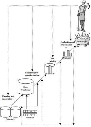
Data Mining is one of the key steps of the Knowledge Discovery process (see Figure 2). After being selected, treated and processed in previous phases, the data are analysed using a Data Mining technique. The choice of the technique will be influenced by the type of intended results and, for some cases, more than one technique will be necessary to achieve the proposed objectives because the quality and type of the data influences the final results (M. Y. Santos & Ramos, 2009).

Figure 2 - Data Mining as a Step in the Knowledge Discovery Process (Han et al., 2012).

Data Mining can be categorized into a few types of tasks in accordance with the objectives of the work (Hand, Mannila, & Smyth, 2001):

 Exploratory Data Analysis – exploring the data without any clear idea of what to look for;

 Descriptive Modelling – describe all the data usually with density estimation or cluster analysis;

 Predictive Modelling – construction of models that predict the value of one variable knowing the values of other variables;

 Discovering Patterns and Rules – searching for combinations in the data that occur frequently and indicates a pattern;

(28)

2.1.2 - Clustering

The objective of clustering is to identify groups of categories or clusters that divide the analysed data, identifying homogeneous groups of objects. This means that the objects in the same group have to be as similar as possible and objects in different groups have to be as dissimilar as possible, ensuring low inter-cluster similarity and high intra-cluster similarity (Jain, Murty, & Flynn, 1999).

This technique is a non-supervised learning technique because the user does not have any influence in the definition of the clusters. Clusters emerge naturally from the data under analysis using some distance function used to measure the similarity among objects (M. Y. Santos & Ramos, 2009).

One good simple example on how we use clustering in our daily lives is when we do our laundry. In order to keep our clothes with their original colours, we group the white ones, the black ones, the coloured ones, etc. because they have that characteristic in common. This is very important since if we mix the clothes from different groups, they will be ruined in the wash. This task is generally very simple unless we have a white shirt with red stripes and then we do not know for sure in which group to put it. When using clustering techniques in decision making, the clusters are often much more dynamic (sometimes they keep changing everyday) causing the decisions concerning to which cluster an object belongs much more difficult (Berson & Smith, 1997).

The important aspect of this technique is the notion of distance, i.e., how it will be decided whether an object or set of objects is similar to other object or set of objects. This “distance” is not mandatorily a real geographical distance, but a measurement of similarity. This measure can be obtained directly from the objects in study or through vectors of characteristics describing each object (Hand et al., 2001). To compute these distances, a “distance function” is defined to measure if an object is near or far from another (Rinzivillo et al., 2008).

It should be highlighted that clustering is not a standalone technique that gives immediate results. The interpretation of the clusters by the user is an essential part of the clustering task. Only that way, the results have some meaning and value and with that, knowledge (Rinzivillo et al., 2008). As it is an unsupervised technique, the user does not have any real intervention and because of that, sometimes it is difficult to interpret the final result.

(29)

However, there are some strategies that can be adopted to overcome this problem. Three of the more popular strategies are (Berry & Linoff, 2000):

 Building decision trees that have the clustering result as the target variable;

 Graphical views which are used to verify how the clustering is affected by changes in the input parameters;

 Checking the differences in the distribution of the variables from group to group, analysing one variable at a time.

2.1.2.1 - Clustering Types

Before explaining some of the approaches the authors use to cluster spatial and spatio-temporal data, it is important to describe the clustering approaches. The clustering technique, according to the majority of the authors, is divided in four main categories (Halkidi, Batistakis, & Vazirgiannis, 2001; Han et al., 2012):

 Partition Clustering;

 Hierarchical Clustering;

 Density-based Clustering;

 Grid-based Clustering.

In the first category (Partition), the dataset is decomposed into a set of clusters. The number of clusters is determined by a k number (parameter given by the user) that optimises a certain criterion function. Each cluster must contain at least one object and each object belongs to exactly one or none group, i.e., the same object cannot be in two groups at the same time.

Most partitioning methods are distance-based and can be divided in two groups: Centroid-based or Representative Object-based techniques. The first one defines the centroid of a cluster as the mean value of the points within the cluster. One of the algorithms used for this technique is the k-means and it is one of the most used clustering algorithms in literature. The second technique derives from the first one. The way the cluster is characterised is defined from a measure (for example, average distance) between a point and the point that defines the cluster. Some of the algorithms used in this technique are: k-Medoids, PAM (Partitioning Around Medoids), CLARA (Clustering Large Applications) and CLARANS (Clustering Large Applications based on Randomized Search) (Han et al., 2012).

(30)

The hierarchical clustering technique groups the data objects into hierarchies or “trees” of clusters. This technique has two different approaches: divisive algorithms and agglomerative algorithms. In divisive, the algorithm starts by considering that all the objects are in one group and, after that, it starts to divide this group in two or more and, also, divide these groups if necessary. This iterative process stops when the maximum number of clusters is reached or the metrics indicate that the set of clusters is the best possible solution. The second strategy is the opposite of the first one. It starts by considering that each object is a group and then integrates clusters to form new clusters. The stopping criteria are the same of the division algorithm (Berry & Linoff, 2000).

The most cited algorithm that uses divisive techniques is CURE (Clustering Using REpresentatives) whilst some algorithms that use agglomerative techniques are BIRCH (Balanced Iterative Reducing and Clustering using Hierarchies), Chamaleon and ROCK (RObust Clustering using linKs) (Halkidi et al., 2001).

Unlike partitioning and hierarchical methods, density-based algorithms identify clusters independently of their shape. Typically, they classify dense regions as clusters and classify regions with low density of objects as noise. To achieve that the algorithms usually look for objects that are near to each other. Some density-based algorithms are SNN (Shared Nearest Neighbour), DBSCAN (Density-Based Spatial Clustering of Applications with Noise), OPTICS (Ordering Points to Identify the Clustering Structure) and DENCLUE (DENsity-based CLUstEring) (Han et al., 2012).

The last technique mentioned is the space-driven Grid-based clustering. In this, the space is divided into a finite number of cells creating a grid structure. After that, all the operations for clustering are done in each cell. Some of the algorithms used in this technique are STING (Statistical Information Grid), WaveCluster and CLIQUE (CLustering In QUEst) (Halkidi et al., 2001).

After analysing the several types of clustering and looking at their main approaches, it is necessary to look at the context of this work, clustering spatio-temporal data, and select the suitable strategy for the analysis of this type of data.

Partition clustering algorithms are applicable mainly to numerical datasets and they cannot handle noise and outliers. Other disadvantage of this approach is that it only discovers

(31)

clusters with convex shape. This type of algorithms needs, as an input parameter given by the user, the number of clusters (Halkidi et al., 2001).

Hierarchical clustering algorithms are, with the exception of BIRCH, are worse than the other types of clustering algorithm in terms of complexity which makes them very slow for large datasets. Instead, BIRCH is faster than the usual hierarchical algorithms but is order sensitive, i.e., with the same input data it may generate different results for different data entry orders. Also, BIRCH does not perform well with clusters of different sizes and shapes (Halkidi et al., 2001).

Density-based algorithms can handle noise, outliers and can create clusters of different sizes and shapes. This type of algorithm generally needs as input parameter the radius of the neighbourhood of a point and the minimum number of points in that neighbourhood. This can be a problem because these parameters are very difficult to determine and the algorithms are very sensitive to them (Halkidi et al., 2001).

Finally, some Grid-based algorithms can detect clusters with arbitrary shape but these techniques do not perform well when clustering high dimensional data. Another problem with this type of algorithm is the ratio efficiency/quality, i.e., in order to have clusters with quality, the simplicity and efficiency of the algorithm has to be compromised (Han et al., 2012).

So, it appears that, for the purpose of this work, the density-based clustering algorithms are the more appropriate technique because (Auria, Nanni, & Pedreschi, 2006; Birant & Kut, 2007; Halkidi et al., 2001; Manso, Times, Oliveira, Alvares, & Bogorny, 2010; Rinzivillo et al., 2008):

 Previous knowledge of the dataset is not required (it does not need the number of clusters as input parameter);

 They can discover clusters with arbitrary shapes such as linear, concave, oval, etc. unlike the classical k-means and hierarchical methods;

 They can process very large databases;

 They can efficiently separate noise in the dataset;

 They have the ability to discover an arbitrary number of clusters to better fit the data under analysis.

(32)

One problem with this type of algorithms is that they require a set of input parameters like the radius of the neighbourhood or the number of neighbours. This problem practically occurs with all types of algorithms and some studies have already been carried out to define heuristics that estimate the values of that input parameters (Ester, Kriegel, Sander, & Xu, 1996; Silva, Moura-Pires, & Santos, 2012).

From the family of the density-based clustering algorithms, the SNN seems to be an appropriate choice for this work because, and unlike the other algorithms in this family, it has the ability to identify clusters of different sizes, shapes and densities. Besides that, in some studies, SNN revealed better results than other density algorithms (Ertoz et al., 2002; Liu et al., 2012; A. Moreira, Santos, & Carneiro, 2005). Although few publications are available about this algorithm, this work tries to contribute to a better understanding of it and to propose extensions that enable it to cluster complex data, as spatio-temporal data.

2.1.2.2 - Shared Nearest Neighbour Algorithm

The SNN algorithm is a density-based clustering algorithm proposed by Ertoz et al. (2002). It has the ability to identify clusters of different (convex and non-convex) shapes, sizes and densities, as well as the ability to deal with noise.

SNN is based on the notion of similarity and defines this similarity between points by calculating the number of nearest neighbours that two points share. The nearest neighbours are calculated using a distance function and the density of a point is the number of points within a given radius. Points with high density are classified as core points and points with low density will become noise points (A. Moreira et al., 2005). This similarity definition between points allows the algorithm to deal with datasets of variable density, being able to identify clusters of different densities (Ertoz et al., 2002).

This algorithm needs three input parameters: k, Eps and MinPts. k is the number of neighbours, Eps defines the threshold density and MinPts is the minimum density that a point has to have to be considered a core point (Ertoz et al., 2002).

The most important input parameter is k (neighbourhood list size) because it strongly influences the granularity of the clusters. If this parameter is too small, even a uniform cluster will be split into several clusters and because of that, the algorithm will have a tendency to find many small, but tight, clusters. On the contrary, if k is too high, the algorithm will find only a few large, well separated clusters. The input parameter MinPts should be a fraction of the number of

(33)

neighbours, k (Ertoz et al., 2002). The importance of these input parameters can be seen in Figure 3 where the k value was set to different values (8 and 12) and the results are very different, ranging from a large set of very small clusters to a small set of very large clusters.

Figure 3 - Clustering Results with Different Values of k (M. Y. Santos, Silva, Moura-Pires, & Wachowicz, 2012).

The main steps of the SNN algorithm are presented next (Ertoz et al., 2002):

1. Construct the similarity matrix: a similarity graph with data points as nodes and edges whose weights are the similarities between those data points;

2. Reduce the similarity matrix: only keep the k most similar neighbours, i.e., the k strongest links of the similarity graph;

3. Create the SNN graph: using the similarity matrix and applying a similarity threshold; 4. Calculate the SNN density of each point: using the Eps value to filter which are

equal or superior;

5. Find the core points: filter points that have density greater than MinPts;

6. Form clusters: if two core points are within a radius, Eps, they are placed in the same cluster;

7. Discard all noise points: all non-core points that are not within a radius, Eps, of a core point are considered noise and consequently, discarded;

8. Assign all the other points to clusters: non-noise and non-core points are assigned to the nearest core point.

For measuring the similarity of data points, a distance function is necessary and, because of the computational complexity, the choice of this distance function is very important. Moreover, the results of this function will greatly influence the clusters so an effective and efficient distance function to help the algorithm is necessary (Lin et al., 2009).

(34)

For example, in spatial data, we could use the Euclidean distance to measure the distance between points. Adding the temporal dimension, 3D vectors of can be used to distinguish between the objects that are near each other in space and time. As can be seen in Equation 1, this distance function can be adapted to the application domain.

Equation 1: √

2.2 - Spatial Data

Nowadays, there is an increasing amount of data about the mobility of people, animals, objects, etc. because tracking systems became more advanced. The number of applications using this type of data are increasing in many areas like (Gonçalves, 2012):

 Search for patterns in human mobility;

 Leisure;

 Optimization of vehicles trajectories (boats, airplanes, etc.);

 Implementation of services based on localization;

 Meteorological services;

 Touristic services;

 Mobile computing.

One good example of how a complex problem can be solved with the use of spatial data is the famous case of John Snow (1855) about the cholera epidemic that emerged in London in the XIX century. More than 500 people died in 10 days and the population got scared. Most of them abandoned the city shortly after, which caused an interruption in the city’s social and economic life.

At that time, nothing about the cause of cholera was known and the general population thought that it had spread through the air, or in a more superstitious way, that it was caused by the vapours of the places where people that died of cholera were buried, two centuries before.

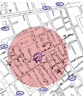
John Snow did not believe that and he was convinced that cholera spread through contaminated water so he registered in a map of London, the number of people that died of cholera and grouped them by houses (example of clustering) and marked the water pumps available to the population. The result can be observed in Figure 4.

(35)

Figure 4 - Map of London by John Snow (1855).

The blue circles are water pumps and the black rectangles are the number of people who died from cholera (the bigger the rectangle, the greater the number). As can be seen, there is a water pump that seems like the epicentre of the epidemic (Broad Street). With this, Snow went to those places and asked where they got the water they used in their daily life and, obviously, all the water was from that particular pump. This case is one of the first documented cases using analysis of spatial data.

Spatial data differs from classical data because unlike the latter, it has coordinate values that refer to a specific reference system. An example of this type of data can be seen in Figure 5.

Figure 5 - Example of Spatial Data.

Spatial data can be represented using three different abstractions of space (Bivand, Pebesma, & Gómez-Rubio, 2008):

 Point: refers to a single point location such as a GPS reading;

(36)

 Polygon: represents an area, outlined by one or more enclosing lines, which may contain holes in it.

The spatial location used in these abstractions is generally related to a position on the Earth’s surface and does not have any temporal information associated with it (Tork, 2012). In spatial data represented by points, sets of vectors are studied that have information about the same characteristics of a given phenomenon in n different locations of a limited spatial domain. An example using points to represent spatial data can be seen in Figure 6.

Figure 6 - Monthly Precipitation in November 2006 (Carvalho & Natário, 2008).

The phenomenon in study is the monthly precipitation in Portugal, measured in millimetres, registered in 158 stations of the national meteorological network during November of 2006. Analysing Figure 6 it is possible to verify that although it was a month of strong rains, its distribution was not uniform. With this type of data, a model can be found for the geographical distribution of precipitation in Portugal that can give some estimation for locals that do not have meteorological stations (Carvalho & Natário, 2008).

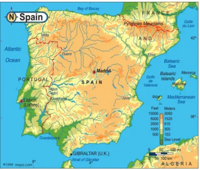
Polygons or areas are used to refer sets of vectors which have data about the same characteristics of a given phenomenon in n sub-regions of a limited spatial domain. This domain is partitioned in various regions, regular or irregular, who have their border well defined using lines (Carvalho & Natário, 2008). In particular, these regions can be created in two different ways, a single categorical variable, such as administrative regions, or a series of attributes like the altitude of the given points as we can see in Figure 7.

Monthly Precipitation (mm) November 2006 • 10 – 130 + 130 – 250 Ο 250 – 370 Δ 370 - 500

(37)

Figure 7 - Map of Altitudes of the Iberian Peninsula (source: www.maps.com).

These two kinds of representation usually use colour stains to classify the valour of the variables in study. The interest in this kind of maps is increasing over the decades because they can give a summarized idea and be easily interpreted, according to the regional distribution (Carvalho & Natário, 2008).

2.2.1 - Spatial Data Mining

Looking at the information that is collected in the organizations every day, some is about addresses, postal codes, geographic coordinates, or simply information stored in a map. The associated spatial component of this kind of data makes it more difficult to analyse because there must be a verification of the spatial relations between the items (such as topological, direction or distance information). The “classic” Data Mining techniques cannot process this kind of data unless there are some modifications that allow them to embody the spatial component. This problem has motivated the appearance of some spatial Data Mining algorithms that allow this kind of systems to deal with spatial data (Maimon & Rokach, 2010).

Spatial Data Mining refers to the extraction of knowledge from spatial data so that it is possible to retrieve information and value from it, as well as, discover spatial relationships and relations between both spatial and non-spatial data (Han et al., 2012).

(38)

2.2.2 - Spatial Clustering

The spatial clustering process is very similar to the “classical” one. It has the same objective (create groups of objects) but the difference is that, in addition to the similarity aggrupation, in spatial clustering, the position of the object is also important. For example, two objects could be very similar but if they are far apart, they will not be in the same cluster if the distance function only uses the geographical position as the similarity measure. So, spatial clustering can be used to combine spatial and non-spatial attributes of the objects.

This technique can be used, for example, to fight crime. Many police agencies are using the benefits of this technology to identify crime hot spots in order to take preventive strategies like intensive patrolling in the detected problematic areas (Maimon & Rokach, 2010).

2.3 - Spatio-temporal Data

Spatio-temporal data refers to a set of objects with their position registered at different time periods (Rosswog & Ghose, 2008). This kind of data has three components: space, time and object. Associated with these components, there are three basic questions that can be answered: space (where), time (when) and object (what) (Andrienko et al., 2011). Unlike spatial data, this type is more complex because the time attribute can be involved in many different ways. Along with the spatial dimension, this type of data has another dimension to classify: the temporal dimension (Kisilevich et al., 2010).

Different forms of spatio-temporal data types are available. They all share the usage of the two dimensions (space and time) but they differ in the amount of information and the way that information is related between dimensions. For point-wise objects, the main classes of spatio-temporal data types are (Kisilevich et al., 2010):

 Events;

 Geo-referenced variables;

 Moving data item or moving objects;

 Geo-referenced time series;

(39)

In spatio-temporal events, there is no relation between the items of the dataset and there is no identification for each data item (or it is not relevant to the study). The spatial and temporal information of the items are both static and, because of that, no movement or any kind of evolution is verified. Each event is usually recorded with the location and the corresponding timestamp. One example of this kind of data is the register of earthquakes by sensors (Kisilevich et al., 2010). A sample of such type of data is presented in Table 1. Using earthquakes as example for the dataset in Table 1, it is possible to see six earthquakes registered (two in each time instant) in six different places.

Table 1 - Sample Dataset of Spatio-temporal Events.

Latitude Longitude Time

X1 Y1 1 X2 Y2 1 X3 Y3 2 X4 Y4 2 X5 Y5 3 X6 Y6 3

The difference between spatio-temporal events and geo-referenced data items is that the latter, in addition to the spatial and temporal dimension, has an associated non-spatial value. Figure 8 presents an example of a dataset of this type of spatio-temporal data. Each point of the dataset in the spatial domain has a timestamp and a semantic attribute value associated.

Figure 8 - Example of Geo-referenced Variables.

The next type is the moving data item or moving object. In such datasets, the items are moving and, therefore, the spatial location of the object is also time-changing. The data generated by moving objects is normally of this kind (id, x, y, t), where id represents the item identifier and x and y are related to the geographical position, usually longitude/latitude based, of

(40)

the object at that time slice (t) (Manso et al., 2010). Usually, datasets with this kind of spatio-temporal data only have the last known location and no trace of the past locations is kept such as real-time traffic monitoring. Figure 9 presents an example of a dataset of this kind where the colour of the point is the identification parameter.

Figure 9 - Example of Moving Objects.

Along with this capability to describe the movement behaviour of the objects, this kind of data can give some other information about the object. The addition of attribute data, which can be static (same value regardless of the position and time, e.g., object type) or dynamic (attribute changes over time, e.g., physical properties such as velocity), is often used in real applications (Mcardle, Tahir, & Bertolotto, 2012).

The two other classes of spatio-temporal data types, geo-referenced time series and trajectories are variations of, respectively, geo-referenced variables and moving objects.

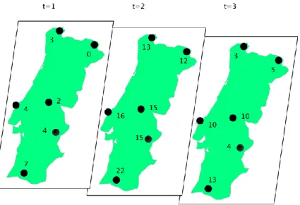
When it is possible to store the attribute variation of an object across time, we have a geo-referenced time series. In this type of data, the spatial dimension of the object stays the same across time whereas the semantic attribute evolves (Kisilevich et al., 2010). This type of data is usually seen in meteorological stations sensors (e.g., temperature or precipitation readings). For example, Table 2 shows the measured temperatures in several cities in three different time instants.

(41)

Conceptual Framework João Ricardo Leite Mota Oliveira Table 2 - Sample Dataset of Geo-referenced Time Series.

Latitude Longitude Time Value

X1 Y1 1 3º X2 Y2 1 0º X3 Y3 1 2º … … … … X1 Y1 2 13º X2 Y2 2 12º X3 Y3 2 15º … … … … X1 Y1 3 3º X2 Y2 3 5º X3 Y3 3 10º … … … …

How this type of data can be represented in a geographical way is presented in Figure 10. For each time period (1,2,3), a different image and different values reflect the values presented in Table 2.

Figure 10 - Example of Geo-referenced Time Series.

Generally, moving objects can be described as trajectories as long as the whole history of the item is stored and available for analysis, i.e., the sequence of spatial positions together with the respective timestamps (Mcardle et al., 2012). One of the main objectives of trajectory clustering is to identify objects with similar movement behaviour, e.g., objects following similar paths in different time periods, objects moving constantly together, etc. (Kisilevich et al., 2010).

A sample of a dataset of trajectories can be seen in Table 3, with the geographical representation presented in Figure 11.

(42)

João Ricardo Leite Mota Oliveira Conceptual Framework Table 3 - Sample Dataset of Trajectories.

ID Latitude Longitude Time

Black X1 Y1 1 Black X2 Y2 2 Black X3 Y3 3 Blue X4 Y4 1 Blue X5 Y5 2 Blue X6 Y6 3 Orange X7 Y7 1 Orange X8 Y8 2 Orange X9 Y9 3 Pink X10 Y10 1 Pink X11 Y11 2 Pink X10 Y10 3 Yellow X12 Y12 1 Yellow X13 Y13 2 Yellow X14 Y14 3 White X15 Y15 3

Figure 11 - Example of Trajectories.

As can be seen, the only thing that enabled us to identify the moving pattern of the object was its identification parameter, specifically the colour in this example. Without it, these items would be spatio-temporal events with no relation with each other.

In this work, the simpler type of object in spatio-temporal data was studied, point-wise objects. There are other types of spatio-temporal data that are spatially more complex such as lines or areas. As the focus of this work is point-wise objects, the other types were not studied in more detail.

(43)

2.3.1 - Spatio-temporal Clustering

The spatio-temporal aspect of the objects involved in the Data Mining process adds more complexity to it. Along with the spatial relations between objects, both metric (like distance) and non-metric (like shape, direction), arises a new relation, the temporal one (like before or after) that needs to be considered in the Data Mining techniques.

This area of study is relatively new and the development of novel algorithms and techniques for the successful analysis of large spatio-temporal datasets is necessary (Rashid & Hossain, 2012).

As a consequence of the emergence of large amounts of spatio-temporal data, aroused the need to analyse that data to discover new knowledge. This brings more complexity to the clustering algorithms because they have to consider both spatial and temporal aspects of the objects in study in order to discover useful knowledge. Even so, the main idea in clustering remains the same, which is to check the characteristics of the objects and to verify which ones are similar and which are not. Spatio-temporal clustering appeared as a new research area in spatio-temporal Data Mining that is growing especially in geographic information sciences, medical imaging and weather forecasting (Birant & Kut, 2007; Kisilevich et al., 2010).

This area will be the focus of the work developed in this thesis and more about the techniques and algorithms that are being used will be presented below.

Various authors have already studied this type of problem and some of them selected the density-based clustering algorithm family but used those algorithms in different ways.

Birant & Kut (2007) created the ST-DBSCAN based on the DBSCAN algorithm (Ester et al., 1996). First, they filtered the spatio-temporal data in order to get the temporal neighbours and their corresponding spatial values and then, applied the algorithm to create the clusters. The authors use the Euclidean distance to measure the spatial distances between points (Eps1) and create another equation, based on the Euclidean distance, to measure the similarity of non-spatial values (Eps2). The data they used to test was composed of locals and temperatures and was in the following format: , where and are the coordenates of the object, in longitude and latitude, and and are, respectively, day time temperature and night time temperature recorded for that position. With another point in the same format (e.g. ), Eps1 and Eps2 are calculated with the following formulas:

(44)

Equation 2: √ Equation 3: √

This implementation can handle temporal aspects as the algorithm first filter the data by retaining only the temporal neighbours and their corresponding values. The authors define that two objects are temporal neighbours if they are in consecutive time units such as consecutive days in the same year or in the same day in consecutive years. This algorithm requires more input parameters (from two to four), adding more complexity to the algorithm tuning process. With this approach the two dimensions (space and time) are not analysed in an integrated way, requiring the application of rules to preselect the data.

Other study (Pöelitz, Andrienko, & Andrienko, 2010) used the DBSCAN algorithm to perform, first, spatial clustering of the data and, then, the temporal clustering of the obtained spatial clusters. The developed approach is also devised for spatio-temporal events. This strategy was followed by Mcardle et al. (2012) to cluster trajectories. They combined both techniques (spatial and temporal) in a very similar way. First, the authors used spatial clustering to extract spatially similar trajectories and then temporal clustering to those clusters was applied. This approach was tested with a dataset containing a relatively low number of records (120 trajectories).

The analysis of the state-of-the-art undertaken allowed the identification of one work that used the SNN algorithm to cluster spatio-temporal data, which is the work of Liu et al. (2012). The authors extended the SNN algorithm and created the STSNN (Spatio-temporal Shared Nearest Neighbour), clustering spatio-temporal events about earthquakes. This algorithm needs a new input parameter ( ), which is added to the three original input parameters of the SNN algorithm (Eps, k, MinPts), allowing the definition of the time window in which two spatio-temporal events are considered neighbours.

For the calculation of the spatio-temporal neighbours, the authors use an abstraction of a cylinder as can be seen in Figure 12.

(45)

Figure 12 - Spatio-temporal Neighbourhood (Liu et al., 2012).

In the centre of the cylinder is the spatio-temporal event to which the neighbours need to be identified. The height of the cylinder is given by and the radius is defined by the windowed distance between the spatio-temporal event and its _{closest spatio-temporal neighbour.}

This algorithm has the following main steps:

 Identify the k spatio-temporal neighbours for each spatio-temporal event;

 For each spatio-temporal event, search the spatio-temporal shared nearest neighbours;

 Calculate the spatio-temporal density of each spatio-temporal event and detect the core ones;

 Expand the clusters by selecting the core events and employing, for each one, a recursive strategy to add all events which are temporal reachable and spatio-temporal connected;

 Identify noise events.

The authors tested their algorithm with different input parameters and concluded that the value of MinPts is dependent and can be a percentage of k. This percentage, according to the several tests done by the authors, should be around 0,5k.

The authors compared the results of the STSNN with the ST-DBSCAN and concluded that the latter cannot find two adjacent clusters with different densities at the same time whereas the STSNN can.

There are other works that use density-based clustering algorithms in other ways like Rinzivillo et al. (2008) who used the OPTICS algorithm (Ankerst, Breunig, Kriegel, & Sander, 1999) to cluster progressively. In this work, the authors created multiple distance functions and

(46)

different input parameters and employed them in a progressive way in accordance to the analysis objective. This approach requires that the analyst or domain expert progressively applies different distance functions to gain understanding of the data in a stepwise manner.

To cluster moving objects, Laube, Kreveld, & Imfeld (2005) created a new concept, the REMO-matrix (Figure 13). In this analysis matrix, the motion of the object is recorded at regular intervals of time and then transformed into angles. After that, these angles are matched to the generic motion patterns proposed by the authors: Constance, Concurrence and Trend-setter.

Figure 13 - The REMO Process (Laube et al., 2005).

Applying these patterns to the movement of people or animals allows the identification of tracks, flocks or leadership patterns, respectively. To identify these patterns it is necessary to calculate the spatial proximity between moving point objects as many objects can move in a similar way but be far from each other not representing any kind of moving pattern between the objects.

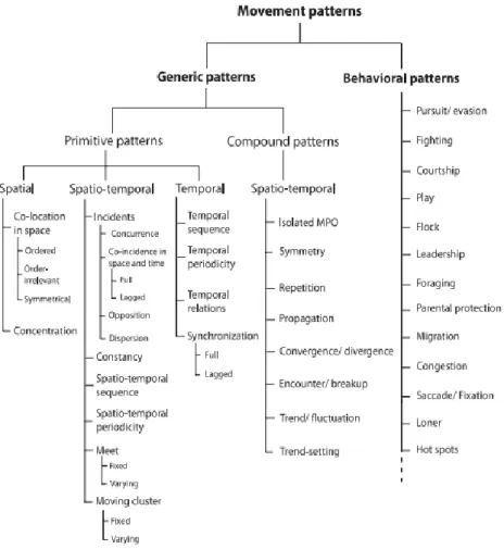
To be possible the identification of moving patterns it is necessary to understand the types of patterns that may exist in real world datasets. Several moving patterns have been described in the literature. The work of Dodge et al. (2008) proposes a taxonomy for the classification of the movement patterns suggesting that those patterns should be applicable to all known types of movement in the human, animal and objects domain (Figure 14).

(47)

Figure 14 - Classification of Movement Patterns (Dodge et al., 2008).

Generic patterns are simpler than behavioural patterns because the latter include movement patterns that can only be found in certain types of moving objects (e.g. a certain animal species).

The generic patterns are divided in two types: Primitive and Compound Patterns. The primitive patterns are the most basic form of movement where only a single parameter varies whilst the compound patterns are more complex because they involve inter-objects relations.

For the authors (Dodge et al., 2008), this kind of taxonomies is indispensable for the development of movement pattern recognition algorithms that are required to be effective, efficient and as generic as possible.

(48)

João Ricardo Leite Mota Oliveira 4D+_{SNN: An Approach to Cluster Spatio-temporal Data}

3 - 4D

+

SNN: AN APPROACH TO CLUSTER

SPATIO-TEMPORAL DATA

The 4D+_{SNN intends to be an approach to cluster spatio-temporal data using the SNN}

density-based clustering algorithm thence the SNN initials in the approach name. 4D represents 4 Dimensions and the + symbol in the name means that the approach can treat data with more than 4 dimensions. In other words, the approach in this work will have the ability to cluster datasets with more than 4 dimensions allowing the integration of space, time and one or more semantic attributes in the clustering process. For this to happen, this algorithm has to allow the simultaneous analysis of 4 or more dimensions ensuring that new dimensions can be integrated either adding new attributes to the distance function used by the SNN algorithm or combining several non-spatial attributes in a single semantic one. This algorithm will also be able to deal with different datasets as well as different discovery purposes as the user will have the ability to define the importance of each dimension in the clustering process. This will be done using weights for each dimension in the distance function used by SNN. How these weights work will be explained in detail later in this chapter. Another parameter introduced in the distance function is the normalization parameter that each dimension used in the distance function has to have in order to adapt different scales and units to similar ones so one dimension is not penalised over other.

In order to test the several approaches defined along the project, it was necessary an implementation of the SNN algorithm. Since there are some implementations already available and free to use there was no need to create one tool that could cluster data with SNN from the beginning. From the studied implementations, it was chosen the one implemented by Antunes (2012). The objective of this implementation1 was to improve the processing time of the SNN

algorithm. In order to accomplish that, it was detected that the calculation of the neighbours list was the most inefficient step in the SNN algorithm. To improve the time of that step the author based his implementation in a concept of division of the space in a grid. One positive aspect of