Abstract—Spatio-temporal clustering is a subfield of data mining that is increasingly gaining more scientific attention due to the advances of location-based devices that register position, time and, in some cases, other attributes. Spatio-temporal clustering intends to group objects based in their spatial and temporal similarity helping to discover interesting spatio-temporal patterns and correlations in large data sets. One of the main challenges of this area is the ability to integrate spatial, temporal and other numerical or classification information in a general-purpose approach as well as the capability to integrate, in the previously obtained clusters, newly available data. This paper presents the Dynamic ST-SNN approach in which the user has the possibility to simultaneously analyse several dimensions and incrementally add new-collected data to the existing clusters providing updated clusters.
Index Terms—Spatial Data, Spatio-Temporal Data, Clustering, Density-based Clustering, SNN.
I. INTRODUCTION
ARGE amounts of data are collected using a variety of devices like satellite images, medical equipment, telecommunication devices, and sensor technologies, among many others. Data Mining, and in particular cluster analysis, can help to automate the analysis of such vast amount of data and to identify patterns, models or other tendencies present in data [1].
Spatio-temporal clustering is a subfield of data mining that is increasingly gaining more scientific attention due to the advances of location-based or environmental devices that register position, time and, in some cases, other semantic attributes of objects or sets of objects [2]. Between the techniques usually used to cluster spatial-temporal data are density-based clustering algorithms [3] [4] and, more specifically, the SNN (Shared Nearest Neighbour) algorithm [5], that presents as main advantages the capability of
Manuscript received March 16, 2015; revised March 31, 2015. This work has been supported by FCT, Fundação para a Ciência e Tecnologia, within the Project Scope UID/CEC/00319/2013 and by Novabase Business Solutions with a co-funded QREN project (24822). Also, we would like to thank the Maritime Research Institute in the Netherlands, for making the data available for analysis under the MOVE EU Cost Action IC0903 (Knowledge Discovery from Moving Objects).
Maribel Yasmina Santos is with ALGORITMI Research Centre, University of Minho, Campus de Azurém, 4800-058 Guimarães, Portugal (corresponding author, phone: +351-253-510308; fax: +351-253-510300; e-mail: [email protected]).
João Moura Pires is with the NOVA-LINCS Lab, New University of Lisbon, Quinta da Torre P-2829-516, Lisboa, Portugal ([email protected]).
Guilherme Moreira, Ricardo Oliveira, Fernando Mendes and Carlos Costa are with the ALGORITMI Research Centre, University of Minho, Campus de Azurém, 4800-058 Guimarães, Portugal.
identifying clusters of different (convex and non-convex) shapes, sizes and densities, as well as the capability to deal with noise. SNN does not require the specification of the number of clusters as an input parameter. In SNN, the notion of similarity is based on the number of neighbours that two points share, value that is computed after the identification of the k-nearest neighbours of each point. The nearest neighbours are identified adopting a specific distance function. In spatial data, the distance function usually includes the Euclidean distance or the Geographical distance. SNN requires three input parameters: k, the number of nearest neighbours that must be identified for each point; Eps, the density threshold that establish the minimum number of neighbours two points should share to be considered similar to each other; and, MinPts, the minimum density that a point should have to be considered a core point. Core points are used to build the clusters.
When clustering spatial data, it is necessary to study the relationship of the objects or entities with the space and, also, the spatial relationships among those objects or entities (like neighbourhood, proximity, among others). With spatio-temporal data, the complexity of the data analysis task increases since those relationships may change with time. Clustering space and time, in an integrated way, requires the analysis of the spatial dimension and the temporal dimension. Moreover, in some application domains, it can be relevant to include in the clustering process semantic attributes that describe properties of the objects. The 4D+SNN algorithm [6] has the ability to weight the importance of each dimension (space, time and semantic dimensions) in the discovery process, allowing the user to deal with different data sets and different discovery purposes.
To allow the updating of the clustering results, as data are progressively collected as time passes, incremental clustering approaches are required. The Dynamic ST-SNN approach proposed in this paper combines the ability to cluster several dimensions with an incremental strategy that dynamically maintains the clustering results updated. Another important characteristic of the Dynamic ST-SNN algorithm is that specific guidelines are used to tune the clustering input parameters [7], strongly reducing the usual trial and error process in which the user continuously changes the input parameters until the results satisfy the analytic requirements.
This paper is organised as follows. Section II presents the related work. Section III describes previous work used in the proposal of the Dynamic ST-SNN approach, which is described in Section IV. Section V evaluates the algorithm while Section VI presents the analysis of a real dataset.
Geo
-Spatial Analytics using the Dynamic
ST
-
SNN Approach
Maribel Yasmina Santos, João Moura Pires, Guilherme Moreira, Ricardo Oliveira, Fernando Mendes
and Carlos Costa
Section VII concludes with some remarks. II. RELATED WORK
For the analysis of spatio-temporal data, using clustering algorithms, several approaches have been proposed. Birant and Kut proposed the ST-DBSCAN [8] based on the DBSCAN algorithm [9]. First, ST-DBSCAN filters the spatio-temporal data in order to identify the temporal neighbours and their corresponding spatial values. Afterwards, the DBSCAN algorithm is applied to form the clusters. The authors use the Euclidean distance to measure the spatial distance between points and propose another equation, also based on the Euclidean distance, to measure the similarity of non-spatial values. This algorithm requires more input parameters, compared with DBSCAN, adding more complexity to the input parameters tuning process. In this approach, the two dimensions (space and time) are not analysed in an integrated way, requiring a previous temporal selection on the data for spatial analysis.
Other work [10] used the DBSCAN algorithm to perform spatial clustering of the data and the temporal clustering of the obtained spatial clusters. The developed approach is devised also for spatio-temporal events. This strategy was also followed by [11] to cluster trajectories. First, spatial clustering is used to extract spatially similar trajectories and then temporal clustering is applied to the obtained clusters. This is a two-step clustering process in which the second step is influenced by the results obtained in the first step.
Another algorithm that was also extended to analyse spatio-temporal data was the SNN algorithm. Liu, Bi and Yang [12] present the STSNN algorithm to cluster spatio-temporal data and they tested it with data about earthquakes. This algorithm needs a new input parameter (∆T), which is combined with the three original input parameters of the SNN algorithm (Eps, k, MinPts), allowing the definition of the time window in which two spatio-temporal events are considered neighbours. The fixed temporal window influences the clustering result.
As data are progressively collected over time, incremental clustering approaches have been proposed to extend existing algorithms. This area of research is gaining increasing attention due to the ever increasing size of data sets and the need to incorporate database updates without having to mine the entire data set again [1]. Although incremental approaches have not been proposed specifically for spatial data, those can be used if the distance function used to measure the objects’ similarity handles this type of data.
Several incremental approaches have been processed so far like IncrementalDBSCAN [13] and Incremental K-means [14]. Although many other incremental approaches can be found in the literature, next paragraphs will focus on density based ones, namely in those that address the DBSCAN algorithm, due to the similarity between DBSCAN and SNN. Both algorithms share the same advantages, but SNN is able to detect clusters of different densities.
In [13], the first incremental version of DBSCAN, called IncrementalDBSCAN, was proposed. The effects of an update operation are limited only to the neighbourhood of the updated object. IncrementalDBSCAN produces the same result as the non-incremental DBSCAN and performs faster
even for a large number of updates. In the incremental clustering process, inserting new objects requires the analysis of the existing connections and new connections may be established as result of this process. The clustering process can, by this way, be restricted to the new points and to the points affected by them. The insertion of a new point can result in the identification of noise, to the creation of a new cluster, to the absorption of the new point by existing clusters or to the merging of existing clusters.
In [15], the authors propose a more efficient incremental algorithm than IncrementalDBSCAN, which allows adding points in a bulk process as opposed to one data point at a time. This approach uses DBSCAN to cluster the new data and proposes a cluster-merging algorithm that can efficiently merge two sets of DBSCAN clusters, the existing ones and the clusters for the new data.
An incremental version of the SNN algorithm was proposed in [16]. The approach follows a strategy that identifies three types of possible changes when a new point is inserted. Although no details about the proposed implementation are given, the authors mention that their approach has as main disadvantage a high memory usage when compared with the original SNN.
The SNN++[17] is an incremental version of SNN, which is based on the Original SNN [5] maintaining its capabilities of identifying clusters of arbitrary shapes, sizes and densities, as well as handling noise. It uses the same 3 input parameters: k, Eps and MinPts. In a general description, the algorithm executes the clustering of the initial data set using the Original SNN. From this step forward, SNN++ receives new packages of objects that are added to the existing clusters without the need to re-start all the process. The clusters are updated each time new data arrives. In this process, new clusters can emerge or be split as consequence of the new densities.
III. PREVIOUS WORK
As mentioned in the previous section, an incremental version of SNN was proposed in [17], allowing an incremental clustering approach for spatial data. In this paper, this incremental version is extended in order to consider spatio-temporal data and to automatically identify the algorithm input parameters attending to the data available for clustering.
For clustering spatio-temporal data with SNN, the 4D+SNN approach, proposed in [6], is able to cluster spatio-temporal data considering in this process space, time and, one or more semantic attributes. It considers all dimensions simultaneously in the distance function, imposing no restrictions to the clusters that can be found. Considering two objects, p1 (<�!,�!,�!,�!>)
and
p2(<�
!,�!,�!,�!>), the distance between them is measured using Equation 1. Typically, x and y are the spatial coordinates, t the timestamp and a an additional attribute.
4��!,�! =�!∗
!"(!!,!!,!!,!!)
!"#$
+�!∗
!"(!!,!!) !"#$
+ �!∗
!"(!!,!!)
!"#$ (1)
In the 4D function, the user can use any distance function (Ds, Dt and Da) to calculate the differences (respectively, spatial, temporal and semantic attribute) between points. ws,
wt and wa are used to assign a weight to each one of these
components (spatial, temporal and semantic dimensions). To guarantee that these weights are an effective mean for controlling the dimension's relative importance in the distance function, it is necessary that the range of values for all distance components are on the same order of magnitude. One way to achieve that is by normalizing the computed values Ds, Dt and Da, in such a way that Ds/MaxS, Dt/MaxT, Da/MaxA become values of the some order of magnitude when the algorithm is calculating the k-neighbours lists. Without this normalization process, the integrated distance function may become strongly dependent of a single distance component if their values are excessively big that the other distance components are irrelevant. In [6], a method to extract MaxS, MaxT and MaxA from the dataset is proposed. By this way, the user can control the pretended results attending to the analytical context.
For the purpose of this work and for all the results presented next, the spatial distance chosen was the Euclidean distance (2). Equation (3) was used for time and Equation (4) for the semantic attribute.
�� �
!,�! = �!−�! !+ �!−�! !
(2)
�� �
!,�! = �!− �! (3)
�� �
!,�! = �!− �! (4)
IV. DYNAMIC ST-SNN
The Dynamic ST-SNN approach combines the possibility to tune the clustering input parameters between consecutive iterations in an incremental clustering approach with the ability to simultaneously consider several dimensions of analysis when clustering spatio-temporal data. To the best of our knowledge, no other approach simultaneously provides those characteristics. The Dynamic ST-SNN algorithm considers as main steps:
Initial data set
1. Read initial data set from file
2. Calculate the input parameters k, Eps, MinPts, and the distance normalization factors
3. Calculate the k-nearest neighbours of each object 4. Measure the similarities and the densities of all objects
5. Build clusters starting with the representative objects
for each iteration do
6. Read incremental data set from file
7. Calculate the new input parameters k, Eps, MinPts, and the distance normalization factors
8. Calculate the k-nearest neighbours of each new object 9. Measure the similarities and the densities of all objects and identify the objects affected by the newly added data objects
10. Build clusters starting with the representative objects of the affected data objects identified in the previous step
11. Identify border points and noise points by iterating through the remaining points of the affected objects
end for
This approach considers that new data bulks are processed with the new input parameters (more data may require new values for the input parameters) and previously processed points maintain their list of k-nearest neighbours excluding those points that are affected by the new inserted ones, belonging to their list of reflexives. With this approach the clusters are updated without the need to reprocess all points. While in the SNN++ approach the results provided by the non-incremental and incremental approach are the same (as the input parameters are the same), the Dynamic ST-SNN approach provides different results that actually consider the appropriate input parameters for each iteration of the clustering.
The following section presents the evaluation of the Dynamic ST-SNN approach, both considering the quality of the obtained results and the algorithm performance.
V. DYNAMIC ST-SNN EVALUATION
This section presents the experimental results that are performed to evaluate the quality and the performance of the Dynamic ST-SNN. Quality is tested using a synthetic dataset, the t5.8k from Chameleon [18]. Performance is tested using a real dataset. The Dynamic ST-SNN performance is compared to the OriginalSNN [5] using a real dataset (MARIN dataset), which integrates data of shipping movements collected by the Netherlands Coastguard, with a total of 280 000 data points.
A. Quality Evaluation
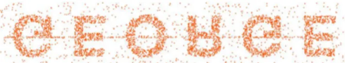
The dataset t5.8k integrates 8000 points as shown in Fig. 1. In this data set, two different modifications (named t5.8k.a and t5.8k.b in this paper) were made for adding the temporal dimension. First (t5.8k.a), the data set was vertically split in six days (one letter per day). For each day, the several points were randomly distributed along the day. To run the Dynamic ST-SNN approach, the t5.8k.a dataset was randomly distributed into three files. The first one, considered the initial dataset, integrates 5 200 points, while the two increments that are going to be used have 1 300 and 1 509 points respectively.
Using the Dynamic ST-SNN implementation, and for t5.8k.a, Fig. 2 shows the result of the first iteration, resulting in 6 clusters, using the same weight for space and time, 50%. Noise points (black points) were identified in the boundary of each time transition. This result shows the adequacy of the distance function defined to measure the similarity of the objects and confirms the correctness of the heuristic applied to identify the variables used in the normalization of each dimension, namely MaxS=0,1985 and MaxT=160. The input parameters used in this first iteration were k=36, Eps=6, MinPts=33, values obtained using the heuristics proposed in [7].
Fig. 2. Quality evaluation, first iteration t5.8k.a (k=36, Eps=6, MinPts=33, ws=50%, wt=50%)
Continuing the incremental clustering, the first increment was added to the previously obtained results allowing the identification of the six letters (Fig. 3), in a picture-perfect identification, using the input parameters k=45, Eps=7 and MinPts=42. Adding the last increment allowed the total rebuilt (Fig. 4) of the dataset, now using the input parameters k=56, Eps=9 and MinPts=52.
Fig. 3. Quality evaluation, first increment t5.8k.a (k=45, Eps=7, MinPts=42, ws=50%, wt=50%)
Fig. 4. Quality evaluation, last increment t5.8k.a (k=56, Eps=9, MinPts=52, ws=50%, wt=50%)
The second transformation (t5.8k.b) was to assign the first four letters to one day and the other two to the following day being the points randomly distributed in each day. The objective is to assign a different temporal behaviour to the dataset forcing the Dynamic ST-SNN approach to deal with the same spatial distribution in a different temporal context. Given this scenario, and in order to be possible the identification of the temporal distribution artificially introduced in the dataset, a weight of 20% for space (ws) and
80% for time (wt) identifies the expected result (Fig. 5) in
the first iteration, as well as in the first and second increments (Fig. 6 and Fig. 7).
Fig. 5. Quality evaluation, first iteration t5.8k.b (k=36, Eps=6, MinPts=33, ws=20%, wt=80%)
Fig. 6. Quality evaluation, first increment t5.8k.b (k=45, Eps=7, MinPts=42, ws=20%, wt=80%)
Fig. 7. Quality evaluation, last increment t5.8k.b (k=56, Eps=9, MinPts=52, ws=20%, wt=80%)
B. Performance Evaluation
The real dataset used to test the performance of the Dynamic ST-SNN is named the MARIN dataset, integrating tracking data of shipping movements collected by the Netherlands Coastguard. This dataset integrates 280,000 data points (Fig. 8).
Fig. 8. MARIN dataset with 280 000 data points
The graphic shown in Fig. 9 compares the runtime for the OriginalSNN and the Dynamic ST-SNN, for a subset of 200,000 points, using incremental steps of 20,000 points. For instance, for 160,000 points, the runtime required by the OriginalSNN to process all the 160,000 points (in just one bulk of data) is slightly higher than the runtime required by the Dynamic ST-SNN to process all the 160,000 points (using incremental additions of 20,000 points). In fact, in all executed experiments, the Dynamic ST-SNN presents a computational pattern almost equivalent or slightly better than the OriginalSNN. These experiments provide empirical evidence that the incremental characteristic of Dynamic ST-SNN was introduced without any computational penalty.
VI. CLUSTERING THE FIRES DATASET
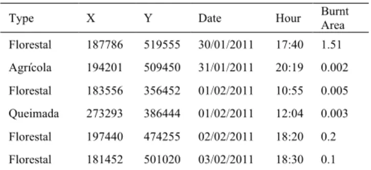
The fires dataset integrates 35,941 fires occurred in Continental Portugal in 2011 with the spatial distribution shown in Fig. 10. Each object in this dataset is described using 38 attributes that include the spatial coordinates; the type of fire; the locality, parish, municipality and district; the date and time of the fire alert; the burnt area; if it was a false alarm; and many other attributes. Table 1 shows an extract of this dataset emphasizing where the fire took place (spatial coordinates), when, its type and the total burnt area.
Fig. 10. Spatial Distribution of the Fires Data Set for 2011.
Table 1. Extract of the FIRES dataset
Type X Y Date Hour Burnt Area
Florestal 187786 519555 30/01/2011 17:40 1.51
Agrícola 194201 509450 31/01/2011 20:19 0.002
Florestal 183556 356452 01/02/2011 10:55 0.005
Queimada 273293 386444 01/02/2011 12:04 0.003
Florestal 197440 474255 02/02/2011 18:20 0.2
Florestal 181452 501020 03/02/2011 18:30 0.1
The temporal distribution per month, during 2011, is also shown in Fig. 10, revealing an usual pattern with many fires in the period from June to September and an unusual behaviour during October 2011 with more than 10 000 fires. In a general overview, most of the fires were small fires with a burnt area smaller or equal than 2 ha.
The Dynamic ST-SNN was applied to the 2011 Portugal fires dataset, using equal weight for the space and time dimensions and to the burnt area attribute, using the distances of equations (2), (3) and (4), respectively. An incremental approach was used, starting with the data available for the first 6 months of 2011, followed by two increments of three months each. Table 2, summarizes the iteration process and shows, for each iteration: the SNN parameters that were automatically suggested by the Dynamic ST-SNN; the number of found clusters and the number of points that were considered as noise.
Analysing the obtained results, the number of points for the 42 clusters (Table 2) varies from 13 fires in one cluster
up to 3528 fires, with an average of 512 fires per clusters. The clusters with more fires are considered the most meaningful ones, existing 16 clusters that aggregate more than 75% of the fires. The spatial, temporal and burnt area dimensions of those 16 significant patterns are shown in Fig. 11, where a) shows the temporal and South-North perspective and b) shows the spatial perspective.
Table 2. Some data about the iteration process
Iteration Period Objects k Eps MinPts Clusters Noise points Initial
data 6
months 9 446 66 11 62
28 4 010
First iteration
3
months 15 851 177 30 166
37 11 359
Second iteration
3
months 10 644 251 43 235
42 13 804
a)
b)
Fig. 11. Spatial Distribution of the Fires Data Set for 2011
occurred in the summer. Clusters 5 to 9 contain the fires occurred in the northern part of the country, 10 and 11 in the centre and cluster 12 in the south. Clusters 13-16 contain the fires occurred at the beginning of autumn. These clusters only appear in the northern and centre parts of the country.
With the spatial perspective of the results it is possible to verify that clusters 5-16 appear at the coastline of the country and only clusters 1-4 have some fires that occurred at the interior part of Portugal. These clusters (1-4) have fires that occurred in the northern part (coastline and interior) of the country and along all the year. They were created due to their higher values of burnt area compared to the ones mentioned before. Clusters 1, 2, 3 and 4 have respectively burnt areas averages of 2.9, 21.4, 6.1 and 1.8. The other formed clusters have very low values (around 0.02).
The clusters that were not shown in the figures had fires with low burnt areas that occurred at the beginning of the year (winter and spring) and the fires that occurred at the interior of the country.
These results show that the Dynamic ST-SNN is able to identify interesting patterns in real data. It should be noted that in the results presented previously, the user did not have any influence on the results since the input parameters were automatically set and the same weights were assigned for each dimension in the analysis.
The user could easily influence the results by giving a higher weight to a specific dimension in order to gain a different perspective on that dimension.
VII. CONCLUSION
This paper presented an incremental clustering algorithm, the Dynamic ST-SNN, based on the SNN algorithm that is able to simultaneously analyse the spatial and temporal dimensions, and one or more semantic attributes, as well as adjust the algorithm input parameters from one iteration to another. The SNN algorithm presents good results identifying clusters of arbitrary shapes, sizes and densities, as well as handling outliers and noise. The Dynamic ST-SNN maintains these capabilities with the advantage of being able to process new data, integrating these new data in the existing clusters, without the need to re-compute the entirely nearest neighbours’ list and, as consequence, repeat the whole clustering process.
The algorithm was tested in what concerns quality and performance. The quality was measured running the algorithm on a synthetic dataset and comparing the clustering results with the expected result.
The performance was tested using a dataset with real data and the results were compared with the OriginalSNN. Performance tests showed that the Dynamic ST-SNN performed better than the OriginalSNN when new data are added to a dataset. As the number of points increases, the gain also increases.
The analytical capabilities of Dynamic ST-SNN were illustrated on a real dataset, the 2011 Portugal fires dataset. In this experiment, the data was processed incrementally, using auto-tuning for the SNN parameters (k, Eps and MinPts), and the automatic estimation of normalization factors that allow the user to freely express the relative importance of space, time and burnt area. The most
significant clusters found are easily interpreted and reveal interesting spatio-temporal patterns.
REFERENCES
[1] J. Han, M. Kamber, and J. Pei, Data Mining: Concept and Techniques. Morgan Kaufmann Publishers, 2012.
[2] S. Kisilevich, F. Mansmann, M. Nanni, and S. Rinzivillo,
Spatio-temporal clustering. Springer, 2010.
[3] A. Moreira, M. Y. Santos, M. Wachowicz, and D. Orellana, “The Impact of Data Quality in the Context of Pedestrian Movement Analysis,” in Geospatial Thinking, M. Painho, M. Y. Santos, and H. Pundt, Eds. Springer Berlin Heidelberg, pp. 61–78.
[4] M. Y. Santos, J. P. Silva, J. Moura-Pires, and M. Wachowicz, “Automated traffic route identification through the shared nearest neighbour algorithm,” in Bridging the Geographic Information Sciences, Springer, 2012, pp. 231–248.
[5] L. Ertöz, M. Steinbach, and V. Kumar, “Finding clusters of different sizes, shapes, and densities in noisy, high dimensional data.,” in SDM, 2003, pp. 47–58.
[6] R. Oliveira, M. Y. Santos, and J. M. Pires, “4D+SNN: A Spatio-Temporal Density-Based Clustering Approach with 4D Similarity,” in Proceedings of the International Conference on Data Mining Workshops, 2013, pp. 1045–1052.
[7] G. Moreira, M. Y. Santos, and J. Moura-Pires, “SNN Input Parameters: how are they related?,” in Parallel and Distributed Systems (ICPADS), 2013 International Conference on, 2013, pp. 492–497.
[8] D. Birant and A. Kut, “ST-DBSCAN: An algorithm for clustering spatial–temporal data,” Data & Knowledge Engineering, vol. 60, no. 1, pp. 208–221, Jan. 2007.
[9] M. Ester, H.-P. Kriegel, J. Sander, and X. Xu, “A Density-based Algorithm for Discovering Clusters in Large Spatial Databases with Noise,” in Proceedings of the Knowledge Discovery in Databases (KDD) Conference, 1996.
[10] C. Poelitz, G. Andrienko, and N. Andrienko, “Finding arbitrary shaped clusters with related extents in space and time,”
Proceedings of the International Symposium on Visual Analytics Science and Technology, 2010.
[11] G. McArdle, A. Tahir, and M. Bertolotto, “Spatio-temporal clustering of movement data: An application to trajectories generated by human-computer interaction,” ISPRS Annals of Photogrammetry, Remote Sensing and Spatial Information Sciences I-2, pp. 147–152, 2012.
[12] Q. Liu, M. Deng, J. Bi, and W. Yang, “A novel method for discovering spatio-temporal clusters of different sizes, shapes, and densities in the presence of noise,” International Journal of Digital Earth, vol. 7, no. 2, pp. 138–157, Feb. 2014.
[13] M. Ester, H.-P. Kriegel, J. Sander, M. Wimmer, and X. Xu, “Incremental clustering for mining in a data warehousing environment,” in VLDB, 1998, vol. 98, pp. 323–333.
[14] S. Chakraborty and N. K. Nagwani, “Analysis and Study of Incremental K-Means Clustering Algorithm,” in High Performance Architecture and Grid Computing, 2011, pp. 338–341.
[15] N. Goyal, P. Goyal, K. Venkatramaiah, P. C. Deepak, and P. S. Sanoop, “An efficient density based incremental clustering algorithm in data warehousing environment,” in Proceedings of the 2009 International Conference on Computer Engineering and Applications, 2009.
[16] S. Singh and A. Awekar, “Incremental Shared Nearest Neighbor Density Based Clustering,” in Proceedings of the 1st. Indian Workshop on Machine Learning, India, 2013.
[17] F. Mendes, M. Y. Santos, and J. Moura-Pires, “Dynamic Analytics for Spatial Data with an Incremental Clustering Approach,” in
Proceedings of the International Conference on Data Mining Workshops, 2013, pp. 552–559.