Dynamic pricing models for electronic business
Y NARAHARI
1, C V L RAJU
1, K RAVIKUMAR
2and
SOURABH SHAH
31Computer Science & Automation, Indian Institute of Science,
Bangalore 560 012, India
2General Motors India Science Laboratory, Bangalore 560 066, India 3Dept. of Computer Science, Birla Institute of Technology and Science,
Pilani 333 031, India
e-mail: [email protected]; [email protected]; [email protected]
Abstract. Dynamic pricing is the dynamic adjustment of prices to consumers depending upon the value these customers attribute to a product or service. Today’s digital economy is ready for dynamic pricing; however recent research has shown that the prices will have to be adjusted in fairly sophisticated ways, based on sound mathematical models, to derive the benefits of dynamic pricing. This article attempts to survey different models that have been used in dynamic pricing. We first motivate dynamic pricing and present underlying concepts, with several exam-ples, and explain conditions under which dynamic pricing is likely to succeed. We then bring out the role of models in computing dynamic prices. The models sur-veyed include inventory-based models, data-driven models, auctions, and machine learning. We present a detailed example of an e-business market to show the use of reinforcement learning in dynamic pricing.
Keywords. Dynamic pricing; shopbots; pricebots; inventory-based models; data-driven models; reinforcement learning.
1. Introduction
e-Business companies are currently grappling with the complex task of determining the right prices to charge a customer for a product or a service. This task requires that a company know not only its own operating costs and availability of supply but also how much the customer values the product and what the future demand would be [1,2]. A company therefore needs a wealth of information about its customers and also be able to adjust its prices at minimal cost. Advances in Internet technologies and e-commerce have dramatically increased the quantum of information the sellers can gather about customers and have provided universal connectivity to customers making it easy to change the prices. This has led to increased adoption of dynamic pricing and to increased interest in dynamic pricing research.
References in this paper are not cited in journal format
There are several survey papers and general articles dealing with different important topics in dynamic pricing. See, for example, the papers by Bakeret al[3], Bichleret al[2], Dimicco et al[4], Chan, Shen, Simchi-Levi and Swann [5], Elmaghraby and Keskinocak [1], Kannan and Kopalle [6], Elmaghraby [7], Leloup and Deveaux [8], McGill and van Ryzin [9], Smith et al[10], Agrawal and Kambil [11], Reinartz [12], Srivastava [13], Varian [14], and Weiss and Mehrotra [15]. There are also several well known papers that have set the foundations for the dynamic pricing problem. These include the papers by Stigler [16], Stiglitz [17], Varian [18,19], Salop and Stiglitz [20], Gallego and van Ryzin [21], and the book by Shapiro and Varian [22].
There are two features that distinguish our paper from the above papers. First, our paper covers a wide range of issues in dynamic pricing whereas the above papers are more focused discussing specific issues. We have made appropriate use of material from the following papers in writing this review: Bichleret al[2], Reinartz [12], Elmaghraby and Keskinocak [1], and DiMicco, Greenwald, and Maes [4]. Second, we survey models of dynamic pricing with e-business and e-commerce as the backdrop. We have categorized the models into four major categories: inventory based models, data driven models, auctions, and machine learning.
Our paper complements and supplements several other papers appearing in this special issue: combinatorial auctions for electronic business [23], pricing strategies for information goods [24], demand sensing in electronic business [25], data mining in electronic commerce [26], Monte Carlo methods for pricing financial options [27], and perishable inventory man-agement and dynamic pricing using RFID [28].
1.1 Outline of the paper
Section 2 motivates dynamic pricing and presents underlying concepts, with several examples, and explains conditions under which dynamic pricing is likely to succeed. In §3, we provide a review of dynamic pricing research using inventory based models. In §4, we present a brief overview of data driven optimization models for dynamic pricing. Section 5 is devoted to auction based models and §6 is devoted to game theoretic models. In §7, we present machine learning based models. Section 8 deals with a detailed example that shows the use of reinforcement learning in dynamic pricing. We conclude the paper in §9.
2. Introduction to dynamic pricing
2.1 From fixed pricing to dynamic pricing
In summary, there are two developments in electronic business which have resulted in a paradigm shift from fixed pricing to dynamic pricing [2].
(1) Transaction costs for implementing dynamic pricing have been reduced by (1) eliminating the need for people to be physically present in time and space, (2) reducing the search costs and (3) reducing the menu costs of informing the changed prices.
(2) Increased uncertainty and demand volatility has led to increased number of customers, increased number of competitors, and increased amount of information. Dynamic pricing itself leads to increased price uncertainty and companies are finding that using a single fixed price in these volatile Internet markets is ineffective and inefficient.
2.2 Dynamic pricing: Definitions
Dynamic pricing is the dynamic adjustment of prices to consumers depending upon the value these customers attribute to a product or service [12]. In the literature, several alternative terms have been used to describe dynamic pricing. These include flexible pricing and cus-tomized pricing. Dynamic pricing includes two aspects: (1) price dispersion and (2) price discrimination. Price dispersion can be spatial or temporal. In spatial price dispersion, several sellers offer a given item at different prices. In temporal price dispersion, a given store varies its price for a given good over time, based on the time of sale and supply-demand situation.
The other aspect of dynamic pricing is differential pricing or price discrimination, where different prices are charged to different consumers for the same product. There are three types here [29,14].
• First degree (or perfect) differentiation: A producer sells different units of output for differ-ent prices and these prices can differ from person to person. Here, each unit of the good is sold to the individual who values it most highly, at the maximum price that this individual is willing to pay for the item. If the producer has sufficient information about to determine the maximum willingness to pay for each customer, this method will be able to extract the entire consumer surplus from the market.
• Second degree price differentiation: This is also called as nonlinear pricing and means that the producer sells different units of output for different prices but every individual who buys the same amount of the product pays the same amount. Thus prices depend on the amount of the product purchased, but not on who does the purchasing. Examples include quantity discounts and premiums. Another example is public utilities; for instance, the price per unit of electricity often depends on how much is bought.
• Third degree price differentiation: This occurs when the producer sells products to different people for different prices, but every unit of product sold to a given person sells for the same price. Price differentiation is achieved by exploiting differences in consumer valuations. An example is group pricing (senior citizens, students, etc.). Another example is telecom pricing (differential pricing for businesses and households).
Elmaghraby and Keskinocak [1] categorize dynamic pricing methods into two broad cate-gories: Posted price mechanisms and price discovery mechanisms. Under the first category, a product or service is sold at a take-it-or-leave-it price determined by the seller. The posted prices could be dynamic, in the sense that the seller changes prices dynamically over time depending on the time of sale, demand information, and supply availability. In price dis-covery mechanisms, prices are determined through a bidding process. Auctions provide an immediate example.
The phraseflexible pricingis often used to denote dynamic pricing. Bichleret al[2] use this term in a broader sense. They distinguish between differential pricing (different buyers receive different prices based on expected valuations) and dynamic pricing (prices are based on bids by market participants), and use the term flexible pricing to refer to both.
In our paper, we use the term dynamic pricing in a broad sense. It would refer in general to dynamic adjustment of prices to consumers. It would include differential pricing, price dispersion, dynamic posted prices, price discovery etc.
2.3 Examples of dynamic pricing
The airline industry is a common example of deployment of dynamic pricing strategies. The kind of pricing strategy followed here is popularly known as yield management or revenue management [9,10,30]. Essentially, the method here is to dynamically modulate prices over time by adjusting the number of seats available in each pre-defined fare class. Advantage is taken of a natural segmentation in the consumers: business travellers for whom the flight dates and timings are primary and fares are secondary; casual travellers for whom prices are important and the dates/timings are flexible; and hybrids for whom both factors are at an equal level of importance. Yield management systems essentially forecast demand, closely monitor bookings, and dynamically adjust seats available in each segment, so as to maximize profits. This method is currently being practiced in hotel rooms, cruises, rental cars, etc. Boyd and Bilegan [30] survey revenue or yield management techniques to illustrate a successful e-commerce model of dynamic, automated sales enabled by central reservation and revenue optimization systems.
Priceline.com allows travellers to name their price for an airline ticket booked at the last minute and get for example a ticket from Boston to San Francisco at USD 275 instead of the full fare of USD 750. Priceline.com uses complex software that enables major airlines to fill unsold seats at marginal revenues. The business model of Priceline.com is attractive for airlines since it can generate additional revenues on seats that would have otherwise gone unsold. Transactions through Priceline.com do not influence buyers with high willingness to pay since a number of serious restrictions apply to the cheaper tickets.
Auction sites such as Ebay.com and Onsale.com have been successfully running auctions where people participate outbidding one another to purchase computers, electronics, sports equipment, etc. at dynamic prices that are governed by supply-demand characteristics.
other sites that enable used cars to be sold through the web. By identifying product features for which consumers are willing to pay a premium, the Ford motor company has developed a pricing strategy that encourages consumers to purchase more expensive vehicles, resulting in a marked increase in revenue and profits [32]. Similarly, General Motors is set to use the data generated from their Auto Choice Adviser website to come up with revenue maximizing dynamic prices for their cars [33].
In September 2000, Amazon.com experimented with prices on their most popular DVDs. Depending on the supply and demand, the prices on a particular DVD varied over a wide range. Customers found out about this and reacted in anger at what they saw as random prices on a commodity which is plenty in supply. Thus price fluctuations can often lead to reduced loyalty from customers if fairness is not perceived.
Buy.com [34,4] uses software agents to search web sites of competitors for competitive prices and in response, Buy.com lowers its price to match these prices. The pricing strategy here is based on the assumption that their customers are extremely price sensitive and will choose to purchase from the seller offering the lowest price. This has resulted in Buy.com register high volumes of trade, however due to the low prices, the profits are low, often times even negative. This example illustrates that overly simplistic or incorrect model of buyer behaviour can produce undesirable results.
2.4 When will dynamic pricing succeed?
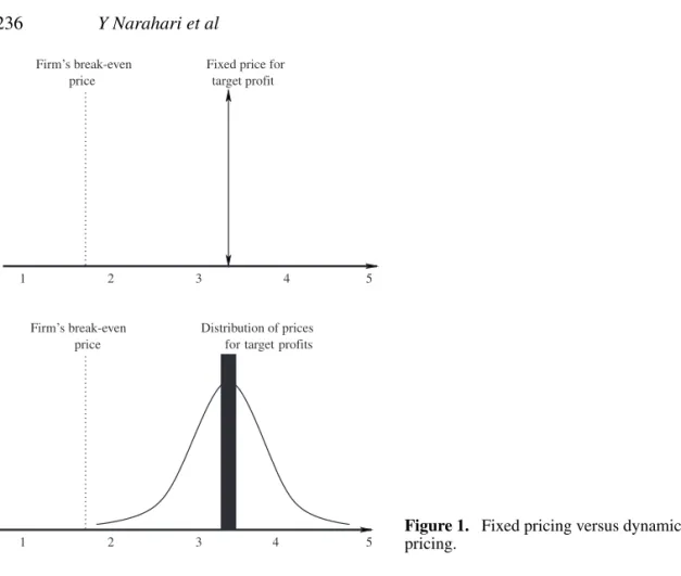
Price customization has become an integral part of electronic commerce these days and is widely accepted. However, the most ideal form of this practice is not yet implemented [12]. A customer’s (buyer’s)willingness to pay(WTP) is the ultimate discriminatory variable (or first degree price customization). See figure 1 [12]. The first part of the figure corresponds to a fixed pricing scenario. Here, the firm will do business with customers 4 and 5 since their WTP exceeds the company’s market price. In the customized pricing scenario (second part of figure 1), there is a distribution of prices with the mean of the distribution converging to the target price. Here, the firm will do business with customers 2,3,4, and 5 since their WTP exceeds the company’s break-even price. Profits will be much higher in the second case.
The difficulty with customized pricing based on WTP is the implementation. Finding out the WTP is not always trivial. Secondly the administrative costs of establishing individual prices can be very high. The advent of the Internet has certainly helped overcome the second difficulty. Technological advances have certainly removed a barrier in implementing dynamic pricing in on-line environments, however a more fundamental question raised by Reinartz [12]. According to him, there are five conditions that must hold for any type of price customization to work, as below.
(1) Customers must be heterogeneous in their willingness to pay, that is they should be willing to pay different prices for the same products or services.
(2) The market must be segmentable, that is, it should be possible to identify different groups of buyers. The web has significantly improved a company’s ability to profile their customers and track their behaviour. Two examples: (1) A grocery customer might sort products by price before choosing (price-sensitive customer) or might use non-price attributes like brand name or quality to shortlist and select (price-insensitive customer). (2) In airlines booking, a business customer is sensitive to the time and date of departure while a price-sensitive customer wishes to choose the minimum price schedule.
Figure 1. Fixed pricing versus dynamic pricing.
For example, a cheaper airline ticket has so many restrictions that to resell it at a higher price is almost impossible.
(4) The cost of segmenting and price differentiation must not exceed revenue due to price cus-tomization. For example, airlines have some of the most sophisticated price customization schemes which took millions of dollars to implement. However, these schemes have led to revenues that are far in excess of the setup costs, leading to the successful deployment of dynamic pricing schemes. Similarly, the presence of companies like Priceline.com has helped the airline industry by generating additional revenues on seats that would have otherwise gone unsold.
(5) Customers should perceive fairness while dealing with a vendor who practices dynamic pricing.
Today’s economy is ready for dynamic pricing, however, the prices will have to be adjusted in fairly sophisticated ways to reap the benefits of dynamic pricing. In the rest of this paper, we look into such dynamic pricing models.
2.5 Models used in dynamic pricing
• Inventory-based models: These are models where pricing decisions are primarily based on inventory levels and customer service levels.
• Data-driven models: These models use statistical or similar techniques for utilizing data available about customer preferences and buying patterns to compute optimal dynamic prices.
• Game theory models: In a multi-seller scenario, the sellers may compete for the same pool of customers and this induces a dynamic pricing game among the sellers. Game theoretic models lead to interesting ways of computing optimal dynamic prices in such situations. • Machine learning models: An e-business market provides a rich playground for online
learning by buyers and sellers. Sellers can potentially learn buyer preferences and buying patterns and use algorithms to dynamically price their offerings so as to maximize revenues or profits.
• Simulation models: It is well known that simulation can always be used in any decision making problem. A simulation model for dynamic pricing may use any of the above four models stated above or use a prototype system or any other way of mimicking the dynamics of the system.
The above way of categorizing dynamic pricing models is in no way a conclusive way. The categorization is neither mutually exclusive nor jointly exhaustive. A certain dynamic pricing scheme may include two or more of the above types. A given type of a model may use another type. For example, inventory based models could be data driven. Machine learning models may be data driven. Machine learning models may use inventory levels in their learning algorithms etc. Simulation is relevant for all the other types of models. In this paper, we provide a brief survey of inventory based models, data driven models, game theory models, and machine learning models. We also present a detailed example to show the use of reinforcement learning in e-business dynamic pricing. We do not discuss simulation as a separate topic since as already stated, simulation is relevant for all the models.
3. Inventory-based models
Dynamic pricing in retail markets based on inventory considerations has been researched quite extensively. Early works include that of Varian [18] and Salop and Stiglitz [20]. Elmaghraby and Keskinocak [1], Swann [35], and Chan, Shen, Simchi-Levi, and Swann [5] provide a comprehensive review of models of traditional retail markets where inventories are used as the main consideration for determining optimal prices. Many of these results are applicable to e-business markets since most retailers have web-enabled e-business operations. We provide a brief overview of some important results here.
Elmaghraby and Keskinocak [1] discuss three main characteristics of a market environment that influence the type of dynamic pricing problem a retailer faces:
• Replenishment vs no-replenishment of inventory (R/NR): In a given time horizon, whether the seller would make pricing decisions given a fixed amount of inventory or inventory can be replenished over time to supply the demand.
• Dependent vs independent Demand over time: Customers demand of a product may change over time.
According to these authors, most existing markets can be classified under three categories: NRIM (no replenishment of inventory–independent demands–myopic customers), NRIS (no replenishment of inventory–independent demands–strategic customers), and RIM (replenish-ment of inventory–independent demands–myopic customers). Examples of NRIM include fashion apparel or holiday products while RIM situation appears in grocery items, produce, and pharmaceutical products. NRIS category is typical business-to-business procurement. The paper provides a comprehensive review of the literature for the above three categories, summarizing all the important results. Most of the results available are for single seller monop-olistic markets.
Gallego and van Ryzin [21] consider optimal dynamic pricing of inventories with stochastic demand over finite horizon. The assumptions made here are: (1) The market is a monopolist market, (2) the selling horizon is finite, (3) the store has a finite stock of items with no replenishment during the selling horizon, (4) demand decreases in price, and (5) unsold items have a salvage value. Gallego and van Ryzin model the demand as a Poisson process with intensityλ(p)whereλ(p)is increasing inp. By charging priceptat timet, the firm controls the intensity of the demand. They show under suitable assumptions that: (a) more stock and/or longer remaining time to sell goods leads to higher expected revenues; (b) at a given point in time, the optimal price decreases as the inventory increases - conversely, for a given level of inventory, the optimal price rises if there is more time to sell. The optimal pricing policies derived call for continuous updating of prices over time, which may not always be practical. The authors investigate heuristic pricing policies with more stable prices. They also look at the case where prices have to be chosen from a discrete set of allowable prices.
Federgruen and Heching [36] consider the optimal inventory and pricing policy of a seller who faces an uncertain demand where prices are changed periodically over time. In each period, before demand is realized, the seller must decide the quantity to produce,qt, given his starting inventory positionxt, wheretdenotes the number of periods remaining. Equivalently, the seller decides how much of inventoryyt to have on hand at the start of the period. It is found that a base stock list price (BSLP) policy is optimal under a wide range of settings. A BSLP policy is defined as follows: (a) if the inventory at the start of the periodt,xt, is less than some base stock levelbt, produce enough to bring the inventory level up tobt and chargept, (b) ifxt is greater thanbt, produce nothing and offer the product at a discounted price ofpt(xt)wherept is a decreasing function ofxt. When the time horizon is infinity, the authors consider two different objectives. When the seller wishes to maximize expected discounted profits, they find that BSLP is optimal. If the seller wishes to maximize average long run profits, then the optimal pricing policy will be a BSLP policy if prices are allowed to move freely.
Bernstein and Federgruen [37,38] consider inventory based pricing in a two echelon supply chain with random demands. The approach used is based on game theory and is reviewed in §6. Learning Curve Simulator [4] is a market simulator, designed and implemented at the MIT Media Labs, for analyzing inventory based dynamic pricing strategies in markets under finite time horizons and fluctuating buyer demands. It can simulate finite markets, that is markets with a finite time horizon, finite seller inventories, and finite buyer population. It can model a wide variety of buyer behaviours and a wide variety of seller strategies. Using this simulator, DiMicco, Greenwald, and Maes [39,4] compare several inventory based dynamic pricing strategies in a single seller market.
performance in automotive industry. They formulate the dynamic pricing problem as an opti-mization problem maximizing total revenue minus holding costs and production costs subject to inventory constraints and production capacity constraints. The problem turns out to be a min-cost network flow problem with convex cost. Their analysis shows that it is possible to achieve significant increase of revenue with dynamic pricing.
We have described here only a few representative models for inventory based dynamic pricing. The reader is referred to the papers by Elmaghraby and Keskinocak [1], Swann [35], and Chan, Shen, Simchi-Levi, and Swann [5] for more details.
4. Data-driven models
Availability of customer data through e-business web sites has opened up enormous oppor-tunities for revenue enhancing measures. E-business sites such as amazon.com, yahoo.com, and the private marketplaces of all leading manufacturing and service companies accumulate huge amounts of data about customers which they can leverage to improve their revenues and profits. In fact, sophisticated data mining algorithms are being developed to make best use of customer data. See the survey on data mining approaches by Raghavan [26] in this special issue. Dynamic pricing is one of the areas significantly impacted by the availability of customer data and data mining algorithms.
We provide several examples of a data driven approach for dynamic pricing. The first example is that of revenue or yield management which are traditionally are driven by customer data. Airlines and the hospitality industry have adopted these techniques quite successfully. Boyd and Bilegan [30] survey revenue management techniques to illustrate a successful e-commerce model of dynamic, automated sales enabled by central reservation and revenue optimization systems. Morriset al[41] examine the dynamic pricing strategies in the airlines industry by discovering patterns in customer preferences. Two adaptive seller-side pricing strategies are presented and evaluated using a Java-based market simulator, Arena. Using the simulator, reserve pricing strategy and seat releasing strategy are compared with the base case in three conditions of increasing, decreasing, and constant customer demands. The results reveal the fact that, by adjusting the reserve price based on the number of seats sold so far in the simulation, the derivative following nature of the reserve pricing strategy was able to track demand very well and increased the revenue over the base case. In contrast, a myopically optimal strategy of adjusting the number of seats released according to the demand level did not succeed in increasing the revenue, in the airline-bidding scenario. A combination of both of these strategies or new invented strategies was simulated with the fluctuating customer demand levels to achieve finer tuning of both reserve price and number of seats released per day and optimize the revenue generation.
By identifying product features for which consumers are willing to pay a premium, the Ford motor company has developed a pricing strategy that encourages consumers to purchase more expensive vehicles, resulting in a marked increase in revenue and profits [32].
from their Auto Choice Adviser website to come up with revenue maximizing dynamic prices for their cars [33].
Once customer data becomes available through web sites and customer relationship man-agement software, a variety of techniques can be used for analyzing and using this data for determining better ways of pricing. Statistical/machine learning techniques are quite popular here.
5. Auction-based models
Auctions constitute a natural model for dynamic pricing. The outcome of an auction is deter-mined by supply-demand characteristics and therefore the prices as deterdeter-mined by an auction can truly be based on market conditions, provided the bidders reveal their true valuations. Auction mechanisms can be designed to have truth revelation properties and the theory of auctions has a great deal to offer to the area of dynamic pricing. Auctions achieve high rates of Pareto efficiency [2] and exhibit rapid convergence to equilibrium. These features would be very attractive in an environment where large companies are buying direct or indirect materials from suppliers who depend on them for a significant portion of their revenue.
Auctions are now possibly the most popular mechanism for implementing price negotia-tions B2B situanegotia-tions. General Electric has adopted online aucnegotia-tions for most of its procurement operations, conducting more than 6 billion online auctions in 2000 [43], which led to the Internet Weekmagazine awarding the title “e-Business of the Year 2000.” Numerous major companies have either used or are in the process of using auction-based methods or internet-based automated negotiations for their procurement/selling operations. There are many pub-lished case studies of successful deployment of e-auctions in procurement (for example, see [44–46]) and in selling (for example, see the survey by Narahari and Dayama [23]).
Auctions are also easily the most popular dynamic pricing mechanism in B2C situations as shown by the success of ebay auctions, yahoo auctions, amazon auctions, and numerous auction sites for air tickets, used cars, entertainment coupons, hotel reservations, etc.
Auctions can take several forms and each type of auction mechanism would implement a particular type of pricing outcome. Bichler et al[2] have described in detail the role of auctions in dynamic pricing, in the context of e-procurement, e-selling, bid preparation, reverse logistics, etc. For this reason, we do not elaborate on this issue in this paper. A companion paper in this special issue looks at combinatorial auctions [23] which represent an important class of auction mechanisms being employed in e-business situations. The paper by Elmaghraby is a focused survey on auctions and pricing in e-marketplaces [7].
There are excellent surveys on general auctions; for example, see [47–52]. The books by Milgrom [53] and Vijay Krishna [54] are excellent treatises on general auction theory. There is a popular on-line book on auctions by Klemperer [55]. There is a very comprehensive recent book on combinatorial auctions by Cramton, Shoham, and Steinberg [56]. We refer the reader to these and other references cited in this section.
6. Game theoretic models
tool. In fact, game theory provides the foundation for design of electronic markets [51]. Both noncooperative game theory and cooperative game theory are relevant for modelling the dynamic pricing problem in e-business markets.
There are a few studies of using a game theoretic approach for dynamic pricing in e-business markets. For example, Bernstein and Federgruen [37,38] consider the dynamic pricing prob-lem in a two echelon supply chain with one supplier servicing a network of competing retailers under demand uncertainty. They assume a single period model in [38] and a periodic review model in [37] and study an infinite horizon problem in both the cases. In [37], in each period, a retailer faces a random demand whose distribution depends on his own retail price as well as the prices charged by the other retailers. Two versions of the model are considered. In the first model, each retailer incurs backlogging costs on backorders. In the second model, appropriate inventory levels are induced by service level constraints of individual retailers. Assuming that the supplier charges a constant per unit wholesale price, the model is shown to induce a noncooperative game among the competing retailers. It is shown that under a Nash equilibrium of this game, each retailer adopts a stationary retail price and a base stock policy with a stationary base stock level. It is also shown that under a specific set of constant wholesale prices, the aggregate system-wide long-run profits of the supplier and retailers are as large as can be achieved in a fully centralized system.
Game theoretic models have recently been used in the area of pricing of network/internet resources [57]. In network settings, dynamic pricing can be used as an effective means to recover cost, to increase competition among different service providers, to reduce conges-tion, and to control the traffic intensity. Game theoretic models become relevant because the entities in a network are selfish and their interaction can be modelled as a noncooperative or cooperative game. The paper by Cao, Shen, Milito, and Wirth [57] examines the use of leader-follower games, cooperative games, and two person nonzero sum games in modelling the Internet pricing problem. It is shown that models based on cooperative games provide the most realistic way of modelling the Internet pricing problem. Game theoretic models which have been used in the context of Internet pricing [58] and network pricing [59,60] can be applied to e-business contexts in a fairly straightforward way.
7. Machine learning-based models
Machine learning has recently emerged as a popular modelling tool for dynamic pricing in e-business. In a typical market, the environment constantly changes with demands and supplies fluctuating all the way. In such a scenario, it is impossible to foresee all possible evolutions of the system. The amount of information available is also limited (for example, a seller does not have complete information about the pricing of the competing sellers). With learning-based models, one can put all available data into perspective and change the pricing strategy to adapt best to the environment. Data drive approaches for dynamic pricing (see Section 4) can use machine learning techniques for determining dynamic prices.
There is a fair amount of literature available on this approach to dynamic pricing. This literature can be logically classified into: single learning agent models and multiple learning agent models. We will first describe a few models that employ a single learning agent.
7.1 Models with a single learning agent
goods. The first strategy uses a single parameter pricing model and the second one uses a two parameter pricing model. It is shown that a dynamic pricing strategy based on two parameter learning obviously outperforms the one based on one parameter learning. The paper derives analytical methods to determining optimal prices for a model with partial information. Simulations are used to explore a dynamic model in which the seller is uncertain about customer valuations and learns the optimal prices gradually.
Gupta, Ravikumar, and Kumar [62] consider a web-based multi-unit Dutch auction where the auctioneer progressively decrements per unit price of the items and model the problem of finding a decrementing sequence of prices so as to maximize total expected revenue, in the presence of uncertainty with regard to arrival pattern of bidders and their individual price-demand curves. The above decision problem is modelled as a single agent RL in an uncertain non-stationary auction environment. Under the assumption of independent bidder valuations, the authors develop a finite horizon Markov decision process model with undiscounted returns and solve it using a Q-learning algorithm.
Carvalho and Puterman [63] consider the problem of a retailer who has to set the price of a good to optimize the total expected revenue over a period of timeT. When the demand function is known, the situation reduces to a simple stochastic maximization problem. However, when the demand function is not known, the retailer has to rely on uncertain prior information to guide his pricing decisions. In this paper, a parametric model is considered in which the parameters are unknown. For example, aftert days of sale, a seller knows the prices he has set on the precedingt−1 days and can observe the demands on the precedingt−1 days. The model is a simple log-linear regression model, where the logarithm of the demand is a linear function of the price. The seller can learn about the parameters of the demand function and use it to set prices so as to maximize the revenues over a given time horizon. Several pricing rules are studied and compared. It is shown that a one-step look-ahead rule performs fairly robustly for a single seller environment studied.
Leloup and Deveaux [8] consider a web store and apply the dynamic pricing model of Rothschild (1974) [64] to match the pricing problem of the web-store. Using simulations, they study the price dynamics that can appear when all the sellers on a given market follow an optimal pricing policy.
Raju, Narahari, and Ravikumar [65–68] look at electronic retail markets with a single seller (without competition). The seller has an inventory of products which he replenishes according to a standard inventory policy. The seller is the learning agent in the system and uses reinforcement learning to learn from the environment. The problem is to determine dynamic prices that optimize the seller’s performance metric (either long term discounted profit or long run average profit per unit time). Under (reasonable) assumptions about the arrival process of customers, valuations of the customers, inventory replenishment policy, and replenishment lead time distribution, the system becomes a Markov decision process thus enabling the use of RL algorithms. Q-learning algorithm for RL is used to solve the problem. The model and solution methodology can also be used to compute optimal reorder quantity and optimal reorder point for the inventory policy followed. This investigation is carried out for two separate, representative situations:
• A retail market where nonlinear prices are offered to different quantities of the product [66]. This is described in more detail in §7.
7.2 Models with multiple learning agents
We now describe a few representative models that employ two or more learning agents. Ravikumar, Saluja, and Batra [69] study a service market environment with two sellers who compete to service a stream of buyers who are of two varieties, informed and uninformed. They assume that both the sellers follow an RL-based adaptive behaviour and model the system as a general sum Markovian game. They propose an actor-critic type of RL scheme (a variant of the scheme proposed by Konda and Borkar [70]) and provide experimental results on convergence.
Hu [71] studies three different types of pricing algorithms (or pricing agents) in a simulated market. The first agent uses reinforcement learning to determine the prices, by learning an optimal action for one period based on the rewards it receives for that action. The second agent uses a traditional Q-learning method, by learning about Q-values which represent long-term optimal values for the agent’s own actions. The third agent uses a sophisticated Nash Q-learning algorithm, by Q-learning about Q-values which represent long-term Nash equilibrium values for agent’s joint actions. The third agent performs better than the second and the second outperforms the first agent in a simulated market where the agents compete with one another. This shows that learning methods that take future rewards into account perform better than myopic methods. Also, the learning method that takes into account the presence of other agents performs better than the method that ignores other agents.
Greenwald, Kephart, and Tesuaro [72] attempt to understand the strategic pricebot dynam-ics in a multi-seller environment where each seller employs a pricebot that employs a price-setting strategy. They examine four different price-price-setting strategies: game theoretic pricing, myoptimal pricing, derivative following, and Q-learning, which differ in their informational and computational requirements. In homogeneous settings, when all the pricebots use the same pricing algorithm, derivative following approach is shown to outperform game theo-retic pricing and myoptimal pricing. In a market with heterogeneous pricebots, myoptimal and game theoretic pricing outperform derivative following while the Q-learning strategy outperforms all the others.
Kephart and Tesauro [73] study aspects of multi-agent Q-learning in a model market in which two identical, competing pricebots strategically price a commodity. Two fundamentally different solutions are observed: an exact, stationary solution with zero Bellman error con-sisting of symmetric policies, and a non-stationary, broken-symmetry pseudo-solution, with small but non-zero Bellman error. This pseudo-convergent asymmetric solution has no analog in ordinary Q-learning. The authors compute analytically the form of both solutions, and map out numerically the conditions under which each occurs. It is suggested that this observed behaviour will also be found more generally in other studies of multi-agent Q-learning.
of maximizing discounted cumulative profit or long run average profit per unit time. Two situations are investigated:
• Case 1: Here, no seller is aware of the states and prices of other sellers. The Q-learning algorithm is used for the pricebot of a distinguished seller and its performance is com-pared with that of pricebots that employ other adaptive techniques such as the well known derivative following (DF) strategy.
• Case 2: Each seller has information about the states and prices of other sellers. Here, the two seller dynamic pricing problem is modelled as a Markovian game and the problem is formulated in the RL framework.
Related investigations are reported in the papers by Sridharan and Tesauro [76], Tesauro and Kephart [77], and Tesauro [78]. Lawrence [79] considers the problem of pricing a bid by a seller in a multi-seller procurement situation. Machine learning is used by seller agents to learn directly the probability of winning from a database of bid transactions with known outcomes. There are several other papers that use different forms of learning in determining dynamic pricing strategies. These include use of learning in a queueing theoretic setting for Internet pricing [80].
8. An example: Using reinforcement learning for dynamic pricing in an e-business market
In this section, we present a reinforcement learning based approach for dynamic price deter-mination in an electronic market with a single retailer. Specifically, we show how optimal nonlinear dynamic prices can be determined in the presence of stochastic demands, price sen-sitive customers, and inventory replenishments. This discussion is taken from [65,66]. The following is a summary of this section.
• We consider a single seller retail store (such as amazon.com) which sells a designated product and offers nonlinear pricing for multiple quantities in order to encourage volume buying. By making reasonable assumptions on the seller’s inventory policy, replenishment lead times, and the arrival process of the customers, we set up a Markov decision process model for the dynamics of this system. In this model, the actions correspond to the prices offered by the seller for different quantities of product bought. Without loss of generality, we consider the situation where the store announces prices for one unit, two units, and three units of the product.
• We show that the seller can use reinforcement learning strategies to modulate his prices dynamically so as to maximize a chosen performance metric. We consider long run time averaged profit as the performance metric. The seller uses Q-learning to learn the optimal dynamic pricing policy.
• We show that the model and the methodology can be used to provide support for tactical decision making such as determining the optimal reorder quantity and optimal reorder point.
We use the phrasesseller,retailer,retail storeinterchangeably in the following discussion.
8.1 Description of system
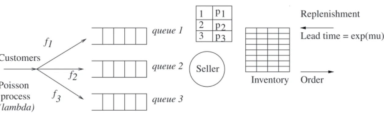
examples. Imagine that the electronic retail store displays a pop-up menu that announces “volume discounts for different volumes of purchase.” We consider, without loss of generality, that the retail store offers three types of packages, one unit, two units, and three units. A customer who clicks on the pop-up menu can be distinguished according to their volume purchases (1, 2, or 3) as type-1, type-2, and type-3 respectively. Also, if the requested item (items) is (are) not present, the store displays a lead time quote for an arriving customer and customers wait for the items if the lead time promised is acceptable. We make the following reasonable assumptions about the system dynamics.
• Customers arrive at the store according to a Poisson process with rate, λ. On arrival, a customer looks at the menu displayed and self-selects her purchase volume. We assume for our analysis that an arriving customer is of type-1 (that is, decides to purchase only one unit) with probabilityf1, of type-2 (that is, decides to purchase two units) with probability f2, and of type-3 (that is, decides to purchase three units) with probability(1−f1−f2). Effectively, this would mean that the arrivals of type-c(c=1,2,3) customers constitute a Poisson process with ratefiλ, wheref3 =(1−f1−f2).
• The seller maintains a finite inventory of the product. Imax is the maximum inventory capacity at the seller’s store. The seller follows a standard inventory policy for replenishing his inventory: whenever the inventory position (current inventory level at the retail store plus the quantity of items ordered as replenishment) drops to a level less thanr (called the reorder point), he would order a replenishment of size(Imax−r). Note that this is a subtle variation of the classical(q, r)inventory policy [81], withq=Imaxand stochastic replenishment time.
• When the number of items requested by waiting customers increases beyond a limit, say N, the seller applies an admission control policy and turns away customers until such time adequate replenishments arrive and the number of items for which customers are waiting decreases to less thanN.
• At any given timet, the seller posts a menu consisting of the following pricing options: a pricepcfor customer type-c. Seller considers pricep1as base price. The seller choosesp2 (p3) in the following way. First, a uniformly distributed price range is chosen forp2 (p3) by picking the upper and lower limits for the uniform distribution asp1b2min andp1bmax2 (p1b3min andp1b3max), whereb2min, b2max(bmin3 , b3max) are price bounds for choosingp2(p3). The base pricep1is dynamically changed by the seller depending on the environment. In fact, this is the central issue in this paper: how does the seller choosep1in response to the events in the system so as to maximize his profits?
• The replenishment lead time (time elapsed between placement of a replenishment order and the arrival of the items) is exponentially distributed (with mean, say, 1/µ).
• We assume that the lead time quotewprovided by the seller for all customers is always the mean of the replenishment lead time, that is, 1/µ. This assumption is justified by the inventory policy that we are using.
• An arriving customer of type-cmeasures her utility of a price quotepcand lead time quote
wby:
Uc(pc, w)=[(1−β)(pc−pc)+β(wc−w)]2(pc−pc)2(wc−w), (1)
where2(x) = 1 ifx ≥ 0 and is zero otherwise, and 0 ≤β ≤1.pc ∼ U (0, pc max] and wc ∼U (0, wc
max] withU (.)denoting the uniform distribution over the specified interval for givenpmaxandwmax.
• If customers of multiple types are competing for items, we choose a customer of a given type with equal probability.
• When a customer arrives into the system, there is a certain amount of time required for her to get the quotes and to decide whether to stay on or leave the system. We assume that this duration is very small and equal to zero. One can assume an infinite server queue to model this initial setup process, however, since that does not offer any more insights into system behaviour, we safely assume the duration to be negligible. Similarly, once an item is available, we assume a waiting customer would immediately take away the item, which means we assume that the time taken for payment and packing is negligibly small. This assumption also does not affect the system dynamics in a way that negates our analysis. • The seller has a finite number of possible options (from setA) for setting his base pricep1. • The seller incurs an inventory holding costHIper unit per unit time and a back order cost
Hqper unit per unit time. The purchasing cost/unit item isC. The ordering cost is assumed to be negligible.
In this example, the seller is the learning agent. Each time a customer stays on or leaves the system, the seller can learn the environment by observing the response to the dynamic prices. If a customer of type-c decides to stay on, there is an assured reward of pc to the seller. The costs incurred by the seller are: (1) purchasing cost for the items ordered by him, (2) inventory holding cost for items stocked in the inventory, and (3) backorder costs on items for which customers are made to wait. In this setting, we wish to enable the seller to dynamically change the base pricep1optimally. The optimality could be with respect to a carefully chosen performance metric. In this paper, we consider two performance metrics: (1) long term total discounted profit the seller will accumulate (over an infinite time horizon) and (2) long run profit per unit time the seller can make.
8.2 Reinforcement learning-based model
Figure 2. A model of a retail store with three customer segments.
Reinforcement learning procedures have been established as powerful and practical meth-ods for solving decision problems in Markov decision processes [84,85]. RL expects a rein-forcement signalfrom the environment indicating whether or not the latest move is in the right direction. The Markov decision process described above is tailor made for the use of reinforcement learning. The seller is a natural learning agent here. The customers are seg-mented into type 1, type 2, and type 3 in a natural way and the seller can quickly identify them. The seller can observe the queue sizes. He also knows the rewards incumbent upon the entry or exit of customers. These rewards serve as the reinforcement signal for his learning process.
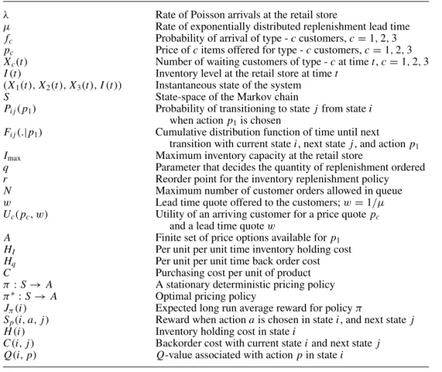
Table 1 describes the notation for the example being discussed.
8.3 System dynamics
The queue, queuec in figure 1, at the retail store is a virtual queue for type-ccustomers. LetX(t ):=(X1(t ), X2(t ), X3(t ), I (t ))be the state of the system at the retailer withXc(.) representing the number of back-logged requests in queue cand I (.), the inventory level at the retailer at timet. The retailer posts unit price quote (p1) and the volume discount alert on his web-page (pricesp2andp3) and will reset the prices only at transition epochs, that is whenever a purchase happens (and hence the inventory drops) or when a request is backlogged in either of the queues. Recall that the customer of type-cwill purchase or make a back log request only whenUcin (1) is positive. It is easy to see that price dynamics can be modelled as a continuous time Markov decision process model. Below we give the state dynamics.
At time 0, the processX(t )is observed and classified into one of the states in the possible set of states (denoted byS). After identification of the state, the retailer chooses a pricing action fromA. If the process is in stateiand the retailer choosesp1∈A, then
(i) the process transitions into statej∈Swith probabilityPij(p1)
(ii) and further, conditional on the event that the next state isj, the time until next transition is a random variable with probability distributionFij(.|p1).
After the transition occurs, pricing action is chosen again by the retailer and (i) and (ii) are repeated. Further, in statei, for the action chosenp1, the resulting reward,Sp(.), the inventory cost,H (i)and the backorder cost C(i, j )costs are as follows: Leti = [x1, x2, x3, i1] and j =[x′
1, x ′ 2, x
′ 3, i
Table 1. Notation for the model of the retail store.
λ Rate of Poisson arrivals at the retail store
µ Rate of exponentially distributed replenishment lead time
fc Probability of arrival of type -ccustomers,c=1,2,3
pc Price ofcitems offered for type -ccustomers,c=1,2,3
Xc(t ) Number of waiting customers of type -cat timet,c=1,2,3
I (t ) Inventory level at the retail store at timet (X1(t ), X2(t ), X3(t ), I (t )) Instantaneous state of the system
S State-space of the Markov chain
Pij(p1) Probability of transitioning to statejfrom statei
when actionp1is chosen
Fij(.|p1) Cumulative distribution function of time until next
transition with current statei, next statej, and actionp1
Imax Maximum inventory capacity at the retail store
q Parameter that decides the quantity of replenishment ordered
r Reorder point for the inventory replenishment policy
N Maximum number of customer orders allowed in queue
w Lead time quote offered to the customers;w=1/µ
Uc(pc, w) Utility of an arriving customer for a price quotepc
and a lead time quotew
A Finite set of price options available forp1
HI Per unit per unit time inventory holding cost
Hq Per unit per unit time back order cost
C Purchasing cost per unit of product
π :S→A A stationary deterministic pricing policy
π∗:S→A Optimal pricing policy
Jπ(i) Expected long run average reward for policyπ
Sp(i, a, j ) Reward when actionais chosen in statei, and next statej
H (i) Inventory holding cost in statei
C(i, j ) Backorder cost with current stateiand next statej Q(i, p) Q-value associated with actionpin statei
Sp(i, a, j )=pc(x
′
c−xc)if x
′
c> xcforc=1,2,3.
=pcif(i1−i
′
1)=c; xc=0 =0 otherwise
C(i, j )=
" 3 X
c=1
c(xc−x
′
c)
++
(i1′ −i1)+
#
C
H (i)= 3
X
c=1
(xcHq)+i1HI
• Remark.Letp1represent the seller’s base price in the observed states. Then the following transitions occur.
– [0, x2, x3, i1]→[0, x2, x3, i1−1] with ratef1λP (U1(p1,µ1) >0) ∀x2, x3andi1 – [0,0, x3, i1] → [0,0, x3, i1 −2] with rate f2λP (U2(p2,µ1) > 0) ∀ x3 and
– [0,0,0, i1]→[0,0,0, i1−3] with ratef3λP (U3(p3,µ1) >0) ∀i1 ≥3 – [x1, x2, x3,0]→[x1+1, x2, x3,0] with ratef1λP (U1(p1,µ1) >0) ∀x2, x3 – [x1, x2, x3,0]→[x1, x2+1, x3,0] with ratef2λP (U2(p2,µ1) >0) ∀x1, x3 – [x1, x2, x3,0]→[x1, x2, x3+1,0] with ratef3λP (U3(p3,µ1) >0) ∀x1, x2.
8.4 Expected long run average reward
Letπ : S → A denote a stationary deterministic pricing policy, followed by the retailer, that selects an action only based on the state information. Lett0 = 0 and let{tn}n≥1 be the sequence of successive transition epochs under policyπ andX(tn−)denote the state of the system just beforetn.
In this case, the performance metric, expected long run averaged reward starting from state ifor the policyπ will be
Jπ(i)=lim sup M→∞
1 MEπ
"M−1 X
n=0
[Sp(X(tn−), π(X(tn−)), X(tn))
−C(X(tn−), X(tn))−H (X(tn−))]|X0 =i
#
. (2)
The retailer’s problem is to findπ∗:S →Asuch that
J∗(i)=max
π Jπ(i). (3)
Let us assume thats is a special state, which is recurrent in the Markov chain for every stationary policy. Consider a sequence of generated states, and divide it into cycles such that each of these cycles can be viewed as a state trajectory of a corresponding stochas-tic maximized profit path problem with state s as the termination state. For any scalar λ, let us consider the stochastic maximized profit path problem with expected stage profit
P
jPij(p)[Sp(i, p, j )−C(i, j )−H (i)]−λfor alli. Now we can argue that if we fix the expected stage profit obtained at stateito beP
jPij(p)[Sp(i, p, j )−C(i, j )−H (i)]−λ∗, whereλ∗is the optimal average profit per stage from state s, then the associated stochas-tic maximized profit path problem becomes equivalent to the initial average profit per stage problem.
Bellman’s equation takes the form:
λ∗+h∗(i)=max p
X
j
Pij[Sp(i, p, j )−C(i, j )−H (i)+h∗(j )], (4)
whereλ∗is the optimal average profit per stage, andh∗(i)has the interpretation of a relative or differential profit for each stateiwith respect to the special states.
8.4a Q-Learning for long run average reward: An appropriate form of the Q-learning algorithm can be written as explained in [86,83], where the Q-value is defined ash∗(i) = maxpQ(i, p),
Qn+1(i, p)=Qn(i, p)+γn[Sp(i, p, j )−C(i, j )−HI(i)Tij−Hq(i)Tij
+max
b Qn(j, b) −max
wherej,Sp(i, p, j ) and C(i, j )are generated from the pair (i, p)by simulation, and Tij is the average sample time taken by the system for moving from state i to state j while collecting samples through simulation. We have to choose a sequence of step sizesγnsuch thatP
γn= ∞and
P
γn2 <∞.
8.5 A simulation experiment
We simulate and study an instance of the retail store model shown in figure 2, by considering an action set (that is, set of possible prices)A= {8·0,9·0,10·0,10·5,11·0,11·5,12·0,12·5, 13·0,13·5}. The maximum queue capacities are assumed to be 10 each for queue 1, queue 2, and queue 3 (this means we do not allow more than 10 of any type of customers in the retail store). The maximum inventory levelImaxis assumed to be 20 with a reorder point atr =10. With these parameter values, the state space of the underlying Markov decision process has 161 states. We assume thatf1=0·4, f2=0·3. We consider customers as arriving in Poisson fashion with mean inter-arrival time 15 minutes. The upper and lower limits for the uniform distribution that describes acceptable price range for type-1 customers are assumed to be 8 and 14, respectively. These limits are assumed to be 12 and 24·5 for type-2 customers and 18 and 35 for type-3 customers. The upper and lower limits for the uniform distribution that describes acceptable lead time range are assumed to be 0 hours and 12 hours, respectively. We consider exponential replenishment lead time for reorders with a mean of 3 hours. The inventory holding cost (HI) is chosen as 0·5 per unit per day and the backorder cost (Hq) is chosen as 8·0 per back order per day. We assume that the seller purchases the items at a unit cost of 4.
We consider the steady state or long run profit per unit time as the performance metric.
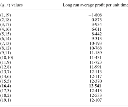
8.5a Optimal values of reorder quantity and reorder point: Assuming the maximum inven-tory capacity at the retail store to be 20, we simulated the system for different values ofq
Table 2. Long run average profit per unit time for different(q, r)values.
(q, r)values Long run average profit per unit time
(1,19) −1·808
(2,18) 0·873
(3,17) 3·934
(4,16) 6·611
(5,15) 8·442
(6,14) 9·313
(7,13) 10·193
(8,12) 10·768
(9,11) 11·189
(10,10) 11·431
(11,9) 11·723
(12,8) 11·991
(13,7) 12·113
(14,6) 12·117
(15,5) 12·370
(16,4) 12·541
(17,3) 12·413
(18,2) 12·533
Table 3. Long run average profit per unit time for a (10,10) policy optimized over different replenishment lead times.
Mean replenishment Cost per unit Long run average lead time (min) for the seller profit per unit time
180 5 10·100
240 4·5 10·922
300 4·25 11·254
360 4 11·431
540 3 9·024
and r in the (q, r) inventory policy used. See table 2. Note thatq is the reorder quantity, whileris the reorder point. From the table, it is clear that a reorder point of 4 and a reorder quantity of 16 are optimal. This means we do not reorder until the inventory position (inven-tory level at the retail store plus the quantity already ordered) goes lower than 4 and when that happens, we place a replenishment order for a quantity of 16. This is a fairly counter-intuitive result, which shows the complex nature of interactions that govern the dynamics of the system.
8.5b Effect of replenishment lead time: We now study the effect of slower or faster replen-ishments. Physically speaking, this is equivalent to ordering replenishments from different distributors. Faster replenishments are naturally associated with higher cost, which is reflected by a higher per unit cost paid by the seller to the distributor. Table 3 provides the results for five different combinations of mean replenishment lead time and cost per unit. The results are quite interesting and show that faster replenishments, even if only marginally more expen-sive, do not guarantee maximization of profit. At the same time, slower replenishments, even if only marginally less expensive, also do not guarantee optimality. Determining the optimal mix of lead time guarantee and per unit cost is a delicate decision that is best left to such models than to plain intuition.
8.6 Optimal nonlinear prices
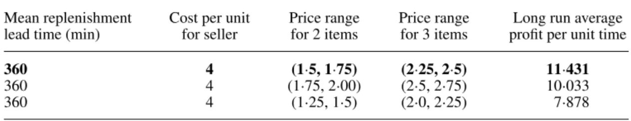
We can use the model to determine the best range of discounted prices to choose for differ-ent quantities, for a given mean replenishmdiffer-ent lead time and cost per unit incurred by the seller. Table 4 shows three different combinations of price ranges for selling 2 items and 3 items. Determining an optimal such combination is best done through a model such as this.
Table 4. Long run average profit per unit time for a(10,10)policy optimized over different price ranges for type-2 and type-3 customers.
Mean replenishment Cost per unit Price range Price range Long run average lead time (min) for seller for 2 items for 3 items profit per unit time
360 4 (1·5, 1·75) (2·25, 2·5) 11·431
360 4 (1·75, 2·00) (2·5, 2·75) 10·033
9. Conclusion
9.1 Summary
It is very clear that advances in internet and e-commerce technologies have opened up rich opportunities for reaping the benefits of dynamic pricing. Companies resorting to dynamic pricing strategies are increasing in number steadily. Moreover, increasingly complex dynamic pricing strategies are being tried out. In this paper, we have covered the following topics.
• We have shown that the fixed pricing paradigm is giving way to a dynamic pricing paradigm in e-business markets and that dynamic pricing strategies, when properly used, outperform fixed pricing strategies.
• We have defined various terms and keywords used in the context of dynamic pricing and provided a categorization of dynamic pricing strategies.
• Conditions under which dynamic pricing strategies will outperform fixed pricing strategies have been enunciated.
• We have categorized and discussed dynamic pricing models under four heads: (1) inventory based models (2) data driven models (3) auction based models (4) machine learning based models based models (2) data driven models (3) auction based models (4) machine learning based models.
• We brought out the role of reinforcement learning based approaches for dynamic pricing and discussed a single seller example with nonlinear pricing used for different quantities.
The main message of this paper is that e-business markets are ready for dynamic pricing, however the prices will have to be modulated in fairly sophisticated ways, based on sound mathematical models, to realize the benefits of dynamic pricing.
9.2 Future work
Current research in this area is focusing on originating increasingly sophisticated methods for dynamic pricing. In the area of auctions, the issue of pricing is closely tied up with truth revelation by bidders. One issue that would need to be studied is how to design truth revealing auction mechanisms that also provide efficient dynamic pricing strategies.
Machine learning based models for dynamic pricing is now an active area of research. The most important problem that requires resolution here is that of multi-agent learning. An equally important issue concerns the computational efficiency of learning based mechanisms. Development of powerful market simulators is another critical area. Real world mod-elling of markets, buying behaviour, seller behaviour, dynamic pricing strategies etc. is an extremely important topic.
*
References
1. W. Elmaghraby and P. Keskinocak. Dynamic pricing: Research overview, current practices and future directions.Manage. Sci.49(10): 1287–1309, October 2003
2. M. Bichler, R.D. Lawrence, J. Kalagnanam, H.S. Lee, K. Katircioglu, G.Y. Lin, A.J. King, and Y. Lu. Applications of flexible pricing in business-to-business electronic commerce.IBM Syst. J.41(2): 287–302, 2002
3. W.L. Baker, E. Lin, M.V. Marn, and C.C. Zawada. Getting prices right on the web.McKinsey Q.10(2): 1–20, 2001
4. J. Morris DiMicco, A. Greenwald, and P. Maes. Learning curve: A simulation-based approach to dynamic pricing, 2002
5. L.M.A. Chan, Z. J. M. Shen, D. Simchi-Levi, and J. Swann. Coordination of pricing and inven-tory decisions: A survey and classification. InHandbook on Supply Chain Analysis: Modelling in the E-Business Era, p 335–392. Kluwer Academic Publishers, 2005
6. P.K. Kannan and P.K. Kopalle. Dynamic pricing on the internet: Importance and implications for consumer behaviour.Int. J. Electron. Commerce, 5(3): 63–83, 2001
7. W. Elmaghraby. Auctions and pricing in e-marketplaces. InHandbook of Quantitative Supply Chain Analysis: Modelling in the E-Business Era. International Series in Operations Research and Management Science, Kluwer Academic Publishers, Norwell, MA, 2005
8. B. Leloup and L. Deveaux. Dynamic pricing on the internet: Theory and simulations.Journal of Electronic Commerce Research, 1(3): 265–276, 2001
9. J.I. Mcgill and G.J. van Ryzin. Revenue management: Research overview and prospects. Trans-portation Science, 33(2): 233–256, 1999
10. B.C. Smith, D.P. Gunther, B.V. Rao, and R.M. Ratliff. E-commerce and operations research in airline planning, marketing, and distribution.Interfaces, 31(2), 2001
11. V. Agrawal and A. Kambil. Dynamic pricing trategies in electronic commerce. Technical report, Stern School of Business, New York University, 2000
12. W.J. Reinartz. Customising prices in online markets.Eur. Business Form6: 35–41, 2001 13. A. Srivastava. Dynamic pricing models: Opportunity for action. Technical report, Cap Gemini
Ernst & Young Center for Business Innovation, 2001
14. H. R. Varian. Differential pricing and efficiency.First Monday, 1, 1996
15. R.M. Weiss and A.K. Mehrotra. Online dynamic pricing: Efficiency, equity, and the future of e-commerce.Virginia J. Law and Technol.11: 1–10, 2001
16. G. Stigler. The economics of information.J. Polit. Econ., 69: 213–225, 1961
17. J. Stiglitz. Equilibrium in product markets with imperfect information.American Econ. Rev. Proc.69: 339–345, 1979
18. H. R. Varian. A model of sales.Am. Econ. Rev.pp 651–659, 1980
19. H. R. Varian. Price discrimination. In R. Schmalensee and R. Willig, editors,Handbook of Industrial Organization. 1989
20. S. Salop and J.E. Stiglitz. The theory of sales: A simple model of equilibrium price dispersion with identical agents.Am. Econ. Rev.72(5): 1121–1130, 1982
21. G. Gallego and G. van Ryzin. Optimal dynamic pricing of inventories with stochastic demand over finite horizons.Manage. Sci.40(8): 999–1020, 1994
22. C. Shapiro and H.L. Varian.Information Rules. HBR Press, Cambridge, MA, 1998
23. Y. Narahari and P. Dayama. Combinatorial auctions for electronic business.Sadhana30: 2005 24. S. Viswanathan and G. Anandalingam. Pricing strategies for information goods.Sadhana30:
2005
25. K. Ravikumar, Atul Saroop, H.K. Narahari, and P. Dayama. Demand sensing in e-business. Sadhana30: 2005
26. N.R.S. Raghavan. Data mining in e-commerce: A survey.Sadhana30: 2005
27. N. Boliya and S. Juneja. Monte carlo methods for pricing financial options.Sadhana30: 2005 28. A. Chande, S. Dhekane, N. Hemachandra, and Narayan Rangaraj. Perishable inventory
man-agement and dynamic pricing using rfid.Sadhana30: 2005 29. A.C. Pigou.The economics of welfare. London: MacMillan, 1920
30. E.A. Boyd and I.C. Bilegan. Revenue management and e-commerce. Manage. Sci.49(10): 1363–1386, October 2003
31. G. McWilliams. Lean machine: How Dell finetunes its pc pricing to gain edge in slow market. Wall Street Journal, June 8, 2001
32. P. Coy. The power of smart pricing.Business Week, April 10 2000
33. P. Rusmevichientong, J. A. Salisbury, L. T. Truss, B. Van Roy, and P. W. Glynn. Opportunities and challenges in using online preference data for vehicle pricing: A case study at general motors. Technical report, Department of Management Science and Engineering, Stanford University, October 2004
34. M. Smith, J. Bailey, and E. Brynjolfsson.Understanding digital markets: Review and assess-ment. MIT Press, Cambridge, MA, 2000
35. J. Swann. Flexible pricing policies: Introduction and a survey of implementation in various industries. Technical Report Contract Report # CR-99/04/ESL, General Motors Corporation, October 1999
36. A. Federgruen and A. Heching. Combined pricing and inventory control under uncertainty. Oper. Res.47: 454–475, 1999
37. F. Bernstein and A. Federgruen. Pricing and replenishment strategies in a distribution system with competing retailers.Oper. Res., 51: 409–426, May-June 2003
38. F. Bernstein and A. Federgruen. Decentralized supply chains with competing retailers under demand uncertainty.Manage. Sci.(to appear), 2005
39. J.M. DiMicco, A. Greenwald, P. Maes. Dynamic pricing strategies under a finite time horizon. InProc. Third ACM Conf. on Electronic Commerce (EC-01)(New York: ACM Press) p 51–60, 2001
40. S Biller, L. M. A. Chan, D. Simchi-Levi, and J. Swann. Dynamic pricing and the direct-to-customer model in the automotive industry.Electron Commerce J.(to appear), 2005
41. J. Morris, P. Ree, and P. Maes. Sardine: Dynamic seller strategies in an auction marketplace. In Proc. Second ACM Conf. on Electronic Commerce (EC-00)(New York: ACM Press) p 128–134, 2000
42. P. Rusmevichientong, B. Van Roy, and P.W. Glynn. A nonparametric approach to multi-product pricing.Oper. Res.(to appear), 2005
43. General Electric Corporation. Letter to share owners. GE Annual Report, 2000
44. W. Elmaghraby and P. Keskinocak. Technology for transportation bidding at the home depot. In Practice of supply chain management: Where theory and practice converge. (Kluwer Academic Publishers) 2003
45. G Hohner, J Rich, Ed Ng, Grant Reid, A J Davenport, J R Kalagnanam, S H Lee, and C An. Combinatorial and quantity discount procurement auctions provide benefits to mars, incorpo-rated and to its suppliers.Interfaces, 33(1): 23–35, 2003
46. J.O. Ledyard, M. Olson, D. Porter, J.A. Swanson, and D.P Torma. The first use of a combined value auction for transportation services.Interfaces, 32(5): 4–12, 2002
47. R.P. McAfee and J. McMillan. Auctions and bidding.J. Econ. Literature, 25: 699–738, 1987 48. P. Milgrom. Auctions and bidding: a primer.J. Econ. Perspect.3(3): 3–22, 1989
49. Paul Klemperer. Auction theory: A guide to the literature.J. Econ. Surv.pages 227–286, 1999 50. J.H. Kagel. Auctions: A survey of experimental research. InThe handbook of experimental
economics(Princeton: University Press) p 501–587 1995
51. J. Kalagnanam and D. Parkes. Auctions, bidding and exchange design. InHandbook of Quan-titative supply chain analysis: Modelling in the e-business era, 2005