Implicit and semiimplicit techniques for the compositional petroleum reservoir simulation based on volume balance

FEDERAL UNIVERSITY OF CEARÁ CENTER OF TECHNOLOGY

DEPARTMENT OF CHEMICAL ENGINEERING GRADUATE PROGRAM IN CHEMICAL ENGINEERING

BRUNO RAMON BATISTA FERNANDES

IMPLICIT AND SEMI-IMPLICIT TECHNIQUES FOR THE COMPOSITIONAL PETROLEUM RESERVOIR SIMULATION BASED ON VOLUME BALANCE

BRUNO RAMON BATISTA FERNANDES

IMPLICIT AND SEMI-IMPLICIT TECHNIQUES FOR THE COMPOSITIONAL RESERVOIR SIMULATION BASED ON VOLUME BALANCE

Thesis presented to the Graduate Program in Chemical Engineering of Federal University of Ceará as a partial requirement for obtaining the Master’s degree in Chemical Engineering. Concentration Area: Chemical Processes. Supervisor: Prof. Dr. Francisco Marcondes. Co-Supervisor: Prof. Dr. Kamy Sepehrnoori.

Dados Internacionais de Catalogação na Publicação Universidade Federal do Ceará

Biblioteca de Pós-Graduação em Engenharia - BPGE

F398i Fernandes, Bruno Ramon Batista.

Implicit and semi-implicit techniques for the compositional Petroleum reservoir simulation based on volume balance / Bruno Ramon Batista Fernandes. – 2014.

167 f. : il. color., enc. ; 30 cm.

Dissertação (mestrado) – Universidade Federal do Ceará, Centro de Tecnologia, Departamento de Engenharia Química, Programa de Pós-Graduação em Engenharia Química, Fortaleza, 2014.

Área de Concentração: Processos Químicos. Orientação: Prof. Dr. Francisco Marcondes. Coorientação: Prof. Dr.Kamy Sepehrnoori.

1. Engenharia Química. 2. Simulação. 3. Volumes finitos. 4. Mecânica dos fluidos. 5. Escoamento em meios porosos. I. Título.

ACKNOWLEDGEMENTS

I would like to express my sincere gratitude to my supervisor, Professor Francisco Marcondes, for all his teaching, guidance, help and patience during these years, and for all the opportunities. I am really grateful for joining his research group. I would like to acknowledge my co-supervisor, Professor Kamy Sepehrnoori, for all his help and opportunities as well. I am grateful for all the helpful comments of Dr. Abdojalil Varavei.

I would like to thank my parents, especially my mother for entrusting her dream of studying for me. I would like to thank my brother for all his fellowship, and for always believing in me.

I would like to express my gratitude to my fiancée, Ana Beatriz Gentil, for all her support, affection, patience, for believing in my potential, and for always standing on my side, even in the bad times.

I thank my friends from the 3D Lab for all their help and fellowship, in special for Pedro Felipe and Victor Aias. I thank my friends, Leonardo Farias and Ítalo Waldimíro, for their fellowship. I would like to thank the friends of the LDFC, in special for Frank Webston for all his help when I joined the group. I acknowledge my friend Dr. Luiz Otávio Schmal dos Santos and his wife, Rubia, for all their help and care during my time at UT Austin, and also with all his important comments for the development of this work.

I would like to express my sincere gratitude to Professor Sebastião Mardônio Pereira de Lucena for all his help and attention towards our group. I also thank the other professors of the Chemical Engineering Department for their teaching, in special for Professor Samuel Jorge Marques Cartaxo.

I thank the members of the qualification and defense committees: Prof. Francisco Marcondes, Prof. Clovis Raimundo Maliska, Prof. Sebastião Mardônio Pereira de Lucena and Prof. Diana Cristina Silva de Azevedo.

I would like to acknowledge the Abu Dhabi National Oil Company, CAPES and PETROBRAS S/A, for the financial support for this research.

“Man would not have attained the possible unless time and again he had reached out for the impossible.”

ABSTRACT

In reservoir simulation, the compositional model is one of the most used models for enhanced oil recovery. However, the physical model involves a large number of equations with a very complex interplay between equations. The model is basically composed of balance equations and equilibrium constraints. The way these equations are solved, the degree of implicitness, the selection of the primary equations, primary and secondary variables have a great impact on the computation time. In order to verify these effects, this work proposes the implementation and comparison of some implicit and semi-implicit methods. The following formulations are tested: an IMPEC (implicit pressure, explicit composition), an IMPSAT (implicit pressure and saturations), and two fully implicit formulations, in which one these formulations is being proposed in this work. However, the literature reports some intrinsic inconsistencies of the IMPSAT formulation mentioned. In order to verify it, an iterative IMPSAT is implemented to check the quality of the IMPSAT method previously mentioned. The finite volume method is used to discretize the formulations using Cartesian grids and unstructured grids in conjunction with the EbFVM (Element based finite volume method) for 2D and 3D reservoirs. The implementations have been performed in the UTCOMP simulator from the University of Texas at Austin. The results of several case studies are compared in terms of volumetric oil and gas rates and the total CPU time. It was verified that the FI approaches increase their performance, when compared to the other approaches, as the grid is refined. A good performance was observed for the IMPSAT approach when compared to the IMPEC formulation. However, as more complex stencils are used, the IMPSAT performance reduces.

RESUMO

Em simulação de reservatórios, o modelo composicional é um dos mais usados para a recuperação avançada de petróleo. Entretanto, o modelo físico envolve um grande número de equações com uma complexa interelação entre elas. O modelo é basicamente composto por equações de balanço e restrições de equilíbrio. A forma como essas equações são resolvidas como, o grau de implicitude, a seleção das equações primárias, variáveis primárias e secundárias tem um grande impacto no tempo de computação. Com o intuito de verificar esse efeito, esse trabalho propõe a implementação e comparação de alguns métodos implícitos e semi-implícitos. As seguintes formulações são testadas: uma IMPEC (implicit pressure, explicit composition), uma IMPSAT (implicit pressure and saturations), e duas formulações totalmente implicitas, das quais uma destas está sendo proposta neste trabalho. Entretanto, a literatura relata algumas inconsistências intrínsecas da formulação IMPSAT mencionada. Para verificar isso, um IMPSAT iterativo foi implementado para verificar a qualidade nos resultados do método IMPSAT préviamente mencionado. O método de volumes finitos é usado para discretizar as formulações usando malhas Cartesianas e não-estruturadas em conjunto com o EbFVM (Element based finite volume method) para reservatórios 2D e 3D. A implementação foi realizada no simulador UTCOMP da Univeristy of Texas at Austin. Os resultados de diversos casos de estudo são comparados em termos das vazões volumétricas de óleo e gás e do tempo total de CPU. Verificou-se que as abordagens totalmente implícitas melhoram sua performance, quando comparado com os demais métodos, a medidaque a malha é refinada. Um bom desempenho foi observado para as formulações IMPSAT quando comparadas com a formulação IMPEC. Entretando, com o uso de conexões mais complexas entre os blocos da malha, o desempho da formulação IMPSAT reduziu.

LIST OF ILUSTRATIONS

CHAPTER 1

Figure 1.1 – Illustration of a typical oil and gas reservoir ... 22

CHAPTER 2 Figure 2.1 – Illustration of the REV ... 38

CHAPTER 3 Figure 3.1 – Cartesian control volume. a) three dimensional view; b) x-y plane view ... 63

Figure 3.2 – Illustration of a dual mesh for the EbFVM approach ... 66

Figure 3.3 – 2D elements in the physical and computational planes. a) Triangle element; b) quadrilateral element ... 67

Figure 3.4 – 3D elements into the physical plane and computational local plane. a) Hexahedron element; b) tetrahedron element; c) prism element; d) pyramid element ... 69

CHAPTER 4 Figure 4.1 – Flowchart of the IMPEC formulation for a time-step ... 76

Figure 4.2 – Flowchart of the IMPSAT-0 formulation for a time-step ... 78

Figure 4.3 – Flowchart of the IMPSAT-1 formulation for a time-step ... 79

Figure 4.4 – Flowchart of the IMPSAT-2 formulation for a time-step ... 81

Figure 4.5 – Flowchart for performing one time-step FI-0 formulation ... 87

Figure 4.6 – Flowchart for performing one time-step for the FI-1 formulation ... 88

CHAPTER 5 Figure 5.1 – Five-spot layout (quarter of five-spot filled). ... 90

Figure 5.2 – 2D Cartesian grids - Case 1. Injectors in blue and producers in red. ... 92

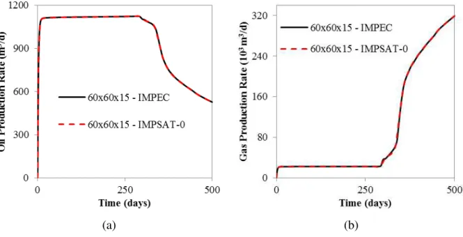
Figure 5.3 – Production rates comparison between IMPEC and IMPSAT-0 – Case 1. a) oil; and b) gas. ... 94

Figure 5.4 – Production rates comparison between IMPEC and IMPSAT-1 – Case 1. a) oil; and b) gas. ... 94

LIST OF TABLES

CHAPTER 1

Table 1.1 – Variables in compositional reservoir simulation. ... 26

Table 1.2 – General concepts of the formulations for compositional reservoir simulation. .... 32

CHAPTER 5 Table 5.1 – Reservoir data for Case 1. ... 90

Table 5.2 – Fluid composition data for Case 1. ... 90

Table 5.3 – Component data for Case 1. ... 91

Table 5.4 – Binary interaction coefficients for Case 1. ... 91

Table 5.5 – Relative permeability data for Case 1. ... 91

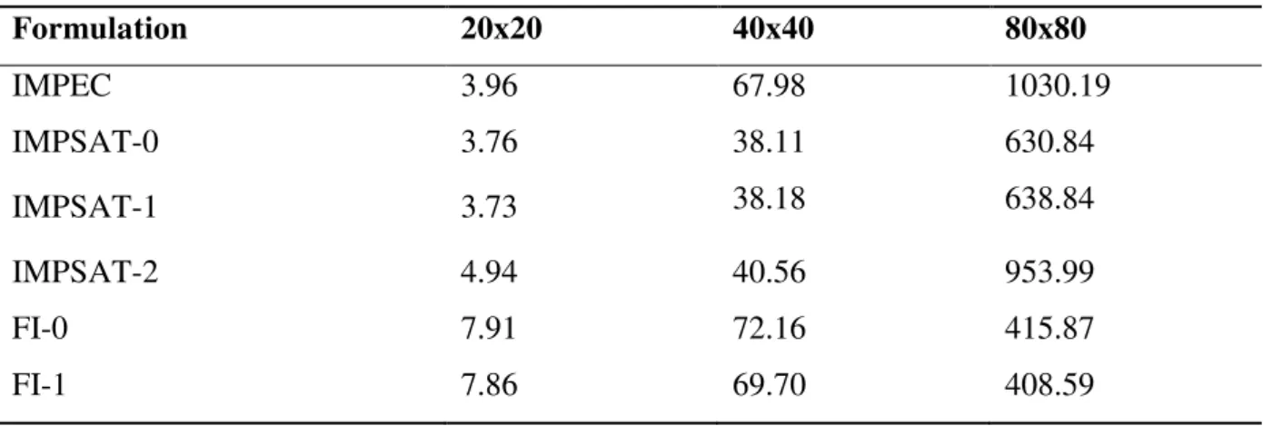
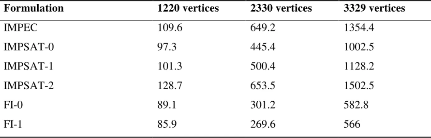
Table 5.6 – CPU time (s) for all simulations - Case 1 using 2D Cartesian grids. ... 102

Table 5.7 – CPU time (s) of all simulations - Case 1 using 3D Cartesian grids. ... 105

Table 5.8 – CPU time (s) of all simulations - Case 1 using 2D regular quadrilateral grids. .. 113

Table 5.9 – CPU time (s) of all simulations - Case 1 using 2D unstructured quadrilateral grids. ... 113

Table 5.10 – CPU time (s) of all simulations - Case 1 using 2D unstructured triangular grids. ... 113

Table 5.11 – CPU time (s) of all simulations - Case 1 using 3D hexahedron grids. ... 122

Table 5.12 – CPU time (s) of all simulations - Case 1 using 3D tetrahedron grids. ... 122

Table 5.13 – CPU time (s) of all simulations - Case 1 using 3D prism grids. ... 123

Table 5.14 – CPU time (s) of all simulations – Case 1 using 3D pyramid grids... 123

Table 5.15 – Reservoir data for Case 2. ... 124

Table 5.16 – Fluid composition data for Case 2. ... 124

Table 5.17 – Component data for Case 2. ... 125

Table 5.18 – Binary interaction coefficients for Case 2. ... 125

Table 5.19 – Relative permeability data for Case 2. ... 125

Table 5.20 – CPU time (s) of all simulations – Case 2. ... 128

Table 5.21 – Reservoir data for Case 3. ... 129

Table 5.22 – Fluid composition data for Case 3. ... 129

Table 5.23 – Component data for Case 3. ... 130

Table 5.24 – Binary interaction coefficients for Case 3. ... 130

Table 5.26 – CPU time (s) for all simulations - Case 3 using a 40x80 2D Cartesian grid. .... 135

Table 5.27 – CPU time (s) for all simulations - Case 3 using a hybrid grid with 3016 vertices. ... 139

Table 5.28 – Reservoir data for Case 4. ... 140

Table 5.29 – Fluid composition data for Case 4. ... 140

Table 5.30 – Component data for Case 4. ... 141

Table 5.31 – Binary interaction coefficients for Case 4. ... 141

Table 5.32 – Relative permeability data for Case 4. ... 141

Table 5.33 – CPU time (s) of all simulations – Case 4. ... 146

APPENDIX A Table A.1. Time-stepping control parameters for Case 1 using 2D Cartesian grids. ... 157

Table A.2. Time-stepping control parameters for Case 1 using 3D Cartesian grids. ... 158

Table A.3. Time-step control parameters - Case 1 using 2D uniform quadrilateral grids. ... 159

Table A.4. Time-step control parameters for Case 1 using 2D unstructured quadrilateral grids. ... 160

Table A.5. Time-step control parameters for Case 1 using 2D unstructured triangular grids. ... 161

Table A.6. Time-step control parameters for Case 1 using 3D unstructured hexahedron grids. ... 162

Table A.7. Time-step control parameters for Case 1 using 3D unstructured tetrahedron grids. ... 163

Table A.8. Time-step control parameters for Case 1 using 3D unstructured prism grids. ... 164

Table A.9. Time-step control parameters for Case 1 using 3D unstructured pyramid grids. . 165

Table A.10. Time-step control parameters for Case 2. ... 165

Table A.11. Time-step control parameters for Case 3 using Cartesian grid. ... 166

Table A.12. Time-step control parameters for Case 3 using the element grid. ... 166

LIST OF ABBREVIATIONS AND ACRONYMS

BF Boundary Fitted CP Corner Point

CV Control-Volume

CVFEM Control Volume Finite Element Method EbFVM Element based Finite Volume Method EOR Enhanced Oil Recovery

EOS Equation of State FEM Finite Element Method FI Fully Implicit

FVM Finite Volume Method IFT Interfacial Tension

IMPEC Implicit Pressure, Explicit Compositions IMPEM Implicit Pressure, Explicit Overall Mass/Moles IMPES Implicit Pressure, Explicit Saturations

IMPSAT Implicit Pressure and Saturations IP Integration Point

MAW Mass Weighted Upwind MCM Multiple Contacts Miscibility

MVNR Minimum Variable Newton-Raphson NOBF Non-Orthogonal Boundary Fitted PEBI Perpendicular Bisector

PREOS Peng-Robinson Equation of State REV Representative Elementary Volume SCV Subcontrol-Volume

SUCV Streamline Upwind Control-Volume TVD Total Variation Diminishing

LIST OF SYMBOLS

a Equation of state parameter.

A Equation of state parameter or area (m2).

b Equation of state parameter or back interface.

B Equation of state parameter or back control-volume.

Cf Formation compressibility (MPa-1).

Cw Water compressibility (MPa-1).

D Depth (m).

e East interface.

E East control-volume.

f Fractionary flow (dimensionless) or fugacity (MPa).

F Volumetric flow rate (m3/d).

g Gravity acceleration (m/d2).

G Gibbs free energy (J).

J Mole flux transported by dispersion (kmol/m2d). L Phase mole fraction (dimensionless).

kr Relative permeability (dimensionless).

K Absolute permeability tensor (m2).

nc Number of components.

np Number of phases.

nj Number of moles of phase j (kmol).

nij Number of moles of component i in phase j (kmol).

nf Number of control volume interfaces.

nv Number of element vertices.

N Total number of moles (kmol) or shape function.

N Total number of moles per pore volume (kmon/m3).

P Pressure (MPa).

Pc Capillary pressure (MPa).

q Mole rate being injected or produced (kmol/d).

S Saturation (dimensionless).

t Time (days).

T Temperature (K) or transmissibility (m3).

U Velocity vector (m/d).

V Volume (m3).

V Partial molar volume (m3/kmol).

w West interface.

W West control-volume.

WI Well index (m3).

x Cartesian coordinate in X direction (m).

xij Mole fraction of component i in phase j (dimensionless).

y Cartesian coordinate in Y direction (m).

z Cartesian coordinate in Z direction (m).

zi Overall mole fraction of component i (dimensionless).

Z Compressibility factor (dimensionless).

Greek letters

ξ Mole density (kmol/m3) or coordinate in the computational plane. Mobility (MPa-1 d-1).

Viscosity (MPa d). ρ Mass density (kg/m3).

η Coordinate in the computational plane. γ Coordinate in the computational plane. ϕ Porosity (dimensionless).

Binary interaction coefficient (dimensionless). ω Acentric factor (dimensionless).

Φ Hydraulic potential (MPa).

Subscripts

b Bulk.

g Gas phase.

o Oil phase.

p Pore or control-volume P.

T Total.

w Water phase or component.

Superscripts

n Previous time-step.

n+1 Current time-step.

m Implicit level to be defined.

SUMMARY

1 INTRODUCTION... 21

1.1 Literature review ... 24

1.1.1 Numerical formulations ... 24

1.1.2 Gridding techniques ... 33

1.2 Layout of this work ... 35

2 MATHEMATICAL MODEL ... 37

2.1 Transport equations ... 37

2.2 Phase behavior ... 44

2.3 Physical properties ... 47

3 APPROXIMATE EQUATIONS ... 60

3.1 Spatial discretization ... 60

3.1.1 Cartesian grid discretization ... 63

3.1.2 EbFVM grid discretization ... 66

3.2 Time-step size selection ... 73

4 FORMULATIONS ... 75

4.1 Ács et al. (IMPEC) ... 75

4.2 Watts (IMPSAT-0) ... 76

4.3 Modified Watts (IMPSAT-1) ... 78

4.4 Iterative IMPSAT (IMPSAT-2) ... 80

4.5 Collins et al. (FI-0) ... 82

4.6 New FI approach (FI-1) ... 87

5 RESULTS AND DISCUSSION ... 89

5.1 Case study 1 ... 89

5.1.1 Case study 1: 2D Cartesian grid ... 92

5.1.2 Case study 1: 3D Cartesian grid ... 103

5.1.3 Case study 1: 2D EbFVM ... 107

5.1.4 Case study 1: 3D EbFVM ... 114

5.2 Case study 2: 2D EbFVM ... 124

5.3 Case study 3 ... 129

5.3.1 Case study 3: 2D Cartesian grid ... 131

5.4 Case study 4: 3D Cartesian ... 140 6 CONCLUSIONS AND FUTURE WORK ... 147

6.1 Future work ... 148 7 REFERENCES ... 149

APPENDICES

1 INTRODUCTION

Petroleum is one of the most important items in the modern society. Not only petroleum is the main energy source in the world, but it is also used as a raw material in countless consumer goods and has numerous applications in industrial processes. The importance of the oil impacts all areas of the society including politics, environment, science, and technology.

Petroleum is a non-renewable mixture of hydrocarbons found naturally in rock formations in the subsurface. Two theories try to explain the origin of these mixtures: the biogenic and abiogenic theories. The biogenic theory, the most accepted one, claims that the hydrocarbon mixtures are formed through the deposition of dead organic matter under lakes and seas through millions of years. During this period, these remains are continuously covered by layers of sediments which become later sedimentary rocks. The heat and pressure under these layers generates innumerous complex chemical reactions converting the organic remains in oil and gas in a very slow process. On the other hand, the abiogenic theory claims that petroleum was formed without the need of biological remains. One of the abiogenic hypothesis, proposed that the petroleum comes from deep carbon deposits as old as the Earth formation. The hydrocarbons then migrate upward reaching the reservoir rocks. Since the biogenic theory has been more successful in the discovery of oil and gas fields, it is much more popular and supported than the abiogenic theory, as concluded by Glasby (2006).

summarized as thermal recovery, gas flooding, chemical injection, among others. The EOR techniques can recover up to 60% (U.S. Department of Energy, 2011) of the original oil in place, while the primary recovery goes up to 20%, and the secondary recovery up to 40% (EPRI, 1999). It is important to mention that these recovered amounts depend on the oil type and reservoir depth.

Figure 1.1 – Illustration of a typical oil and gas reservoir.

monophasic one-dimension flow to two and three dimensions, with multiphase flow in transient regime and heterogeneous media (Coats, 1982a; Coats, 1982b). Before the 70’s, the computational models were mainly based on Black-Oil models. The Black-Oil model assumes that three pseudo-components exist inside the reservoir: oil, gas and water. In general, the gas component can exist in the oil and gas phase, but the oil and water components cannot be transferred to the other phases. Although the Black-Oil model is simple and has a low computational cost, it lacks realism and it is suitable only for heavy oils. The increase in oil prices led to the development of many EOR techniques. These processes could not be modelled with the Black-Oil model unless large errors in the predictions with this model were acceptable. Several models emerged to treat each EOR processes. However these models were soon replaced by multipurpose models that could handle several processes. According to Ács et al. (1985), two reasons led to this: first, the expenses involved in training, development and maintenance of these multiple models; and second, the search for a model which could have a common basis to help surveys and comparisons for the understanding of different oil recovery mechanisms.

The reservoir simulation had a great evolution since its beginning, not only in the physical modelling equations used but also in many other features such as: numerical formulations, gridding, flux approximation schemes, phase behavior calculations, geomechanics models, fractures and fault models and linear solvers.

Solving the equations involved is still a difficult task, consuming even days of computation even with the most modern computers to provide a single result. In order to provide feasible computation times, many algorithms were proposed for all types of models, from black-oil to thermal compositional models, differing in complexity, robustness and consistency. These algorithms are called numerical formulations. Although the development of compositional simulators is underway for more than three decades, this is still a challenging task, given the large number of partial differential equations to be solved and the large number of variables that must be determined. The main goal of this work is to investigate several numerical formulations using Cartesian and unstructured grids, with the goal of evaluating the performance of each formulation in terms of accuracy and overall computational cost for processes like miscible and immiscible gas flooding and CO2 injection for isothermal compositional reservoir simulation.

by IMPEM (Implicit Pressure, Explicit Overall Mass/Moles) (Wong and Aziz, 1989) and IMPEC (Implicit Pressure, Explicit Compositions). The IMPES, IMPEM and IMPEC formulations share the same basis of evaluating in which only pressure is evaluated implicitly and the use of each one of these nomenclatures are used according to the variables that are computed explicitly through the other material balance equations. Since saturation is not a common term in chemical engineering field, it is important to mention that it refers to the volumetric fraction of each phase that resides into the pore volume.

1.1Literature review

A literature review is presented in this section. First, a review of the numerical formulations for isothermal compositional simulation, then a review of the gridding techniques used in reservoir simulation is presented.

1.1.1 Numerical formulations

The physical models used in petroleum reservoir simulation evolved in realism and robustness through time, but they also increased their complexity as a consequence. One of the first models used was the Buckley-Leverett model (1942). This model describes an incompressible/immiscible multiphase flow. Buckley and Leverett (1942) also presented the analytical solution for the two-phase flow of oil and water using this model. Muskat (1949) developed the three-phase Black-Oil model which was improved and modified for several applications in the oil industry being used up to date. The compositional models are relatively more recent. The development of compositional reservoir models was supported by the development of accurate Equations of State (EOS) for the phase behavior of oil and gas calculations. Although the use of EOS increased the computational cost of the models, the use of these models was encouraged by the evolution in the computers’ processing power.

The early compositional models neither used fugacity nor EOS. Physical properties were evaluated through correlations. These simulators presented several convergence problems. Fussel and Fussel (1979) were the first to use an EOS to evaluate properties and phase behavior and have overcome the convergence problems of the previous simulators. Thele (1984) presents a review of the compositional models that did not use EOS.

coupling with the phase equilibrium equations, and the choice of the variables to be solved with the balance equations.

Before looking at the compositional formulations it is necessary to define the concept of primary and secondary variables. The hypothesis of local equilibrium is usually accepted in the field of reservoir engineering and considers that each point of the reservoir is in a thermodynamic equilibrium related to the conditions and overall compositions at that point. This assumption makes valid the Gibbs’ phase rule:

thermo P

F   N 2 N , _(1.1)

where Fthermo is the degree of freedom, NP is the number of phases in equilibrium, and N is the number of components present in the phases in equilibrium. The degrees of freedom are the number of independent intensive parameters that determine the all other intensive variables of the system. Water component is not usually included into flash calculations; therefore there is no mass transfer between the water phase and the other hydrocarbon phases. With these assumptions, the value of N becomes nc and the value of NP becomes np-1, where nc is the number of components excluding water and np is the number of phases existing inside the reservoir. If the model is to be considered isothermal, then one of the independent intensive parameters is fixed and one parameter less needs to be determined. Additionally, in multiphase flow in porous media, it is necessary to determine the phase saturations in order to compute the phase flow; this will include np more independent variables to be determined. However, one saturation can be eliminated with the saturation constraint, which is given by

np

j j

S







1

1. (1.2)

Applying the above assumptions, eliminating one parameter with Eq. (1.2), and substituting it in Eq. (1.1), the number of independent variables reduces to

thermo c

F n 1. _(1.3)

The nc+1 intensive parameters that must be determined are called primary

Table 1.1 – Variables in compositional reservoir simulation.

Variable Definition Total quantity Number

eliminated

Final quantity

Pj Phase pressures. np np-1 1

Sj Phase saturations. np 1 np-1

xij Phase compositions. nc(np-1) np-1 (nc-1)(np-1)

Total: np(nc+2)-nc 2np-1 nc(np-1)+1

As shown in Table 1.1, the total number of variables to be determined are

np(nc+2)-nc. All other properties and parameters involved in a isothermal reservoir simulation considering local equilibrium can be obtained using these variables. Note that quantities in Table 1.1 are taken assuming that water is present only in water phase and the water component cannot be found in any of the hydrocarbon phases. The phase pressures are related to each other through the capillary pressure relations. The capillary pressure relations allow selecting just one phase pressure as a reference and then computing the others from this reference. This eliminates np-1 variables. One of the saturations is also dependent from the others through the saturation constraint and eliminates one more variable, as it was shown previously. Also, the phase compositions of each phase must sum up to one. It adds one more equation to determine the composition for each hydrocarbon phases, therefore np-1 variables can be eliminated. Finally, after the elimination of all depending variables, nc(np-1)+1 variable still remain, as shown in Table 1.1. If the most typical situation in a reservoir is assumed, namely a three phase system (water, oil and gas), then the number of variables becomes 2nc+1. Since the nc+1 primary variables are usually determined from the flow equations, it will be necessary to compute nc(np-2)more variables. These variables are called the secondary variables, and most models use the equilibrium relations to determine them. The equilibrium relations are the isofugacity equations. The equilibrium relations will be discussed later in chapter 2.

Most of the numerical formulations use the concepts of primary and secondary variables. The literature review of the numerical formulations will be now addressed.

and capillary pressure. Additionally, the mass transfer between the hydrocarbon and the water phase was not considered. This formulation differs from all other isothermal compositional formulations since it is the only formulation that uses constraint equations (equilibrium equations and volume constraint) to solve nc+1 primary variables. This formulation is an IMPES-type and uses a Minimum Variable Newton-Raphson (MVNR) method to reduce the number of equations and variables by a Gauss elimination procedure. The primary variables are not fixed and are selected according to the predominance of oil or gas in a given grid block. The phase predominance is determined by verifying which phase has the greater number of moles per pore volume. If liquid phase prevails in a grid block, then the primary variables will be the pressure, the number of moles per pore volume of gas phase and nc-1 compositions of the gas phase {P,

N

_g, x2_g, …,

x

n gc }. On the other hand, if the gas phase

prevails, then the set of variables will be the pressure, the number of moles per pore volume of oil phase and nc-1 compositions of the oil phase {P, N_o, x2_o, …,

x

n o_c }. The authors called the MVRN using the first set of variables by V-Y-P iteration and the MVRN using the second set by L-X-P iteration. All the flow equations of this formulation are based on mole balance equations.

Coats (1980) presented the first FI formulation for the isothermal compositional model. The model considered three dimensions and three phases, and the gravity and capillary pressure effects were taken into account. Furthermore, the capillary pressure and relative permeabilities are considered as functions of saturations and also of the interfacial tensions (IFT). The modified Redlich-Kwong EOS (Zudkevitch and Joffe, 1970) was used by the author for the density and phase equilibrium calculations. This model also does not consider mass transfer between the water phase and the hydrocarbon phases. The primary equations are the nc hydrocarbon material balance equations and the water balance equation. A Newton-Raphson method is used to solve the discretized set of equations, generating a block Jacobian matrix in which each entry has (2nc+1) (2nc+1) size for the two hydrocarbon phases presented into the system. It is worthwhile to mention that primary and secondary variables are coupled into the Jacobian matrix. In order to decouple them, a Gauss elimination approach is used reducing each block of the Jacobian matrix to a (nc+1) (nc+1). The secondary variables are then computed after solving the primary variables. The primary variables for a grid block with both oil and gas phases are the gas phase pressure, oil and gas saturations, and

phase, the primary variables are: {Pg, S_g, x2_g, …,

x

n gc }. If the grid block has only oil phase,

the primary variables will be: {Po, S_o, x2_o, …,

x

n o_c }. The author also mentions that for grid blocks with immobile water, the water saturation is kept constant and one more saturation is eliminated. Coats (1980) treated the phase disappearance verifying the saturation value at the end of a Newton iteration; if a saturation is less than zero, the saturation of the grid-block is set to zero for the next Newton iteration. The phase appearance was treated by calculating a saturation pressure. If the saturation pressure is less than the grid block pressure, then the grid-block is single hydrocarbon phase, otherwise the grid block is considered to have two hydrocarbon phase and the value of the saturation of the absent phase is set to 0.001. The great advantage of the Coats formulation is that most terms of the Jacobian matrix are directly calculated, since most of the primary variables are explicitly in the mole balance equations. Due to this feature, this set of primary variables is normally called the natural variables. On the other hand, the flash procedure is treated in a special way, making impossible to use general flash algorithms. In his paper, the author used the formulation to solve problems of multicontact-miscibility (MCM) problems. According to Coats (1980) these simulations are characterized by a great amount of numerical dispersion.

Nghiem et al. (1981) developed an IMPES-type formulation that differs from the previous ones by solving pressure and compositions separately. Nghiem et al. (1981) considered a three dimensional model with three phase flow. The Peng-Robinson (1976) EOS was used and the effects the IFT were included into the relative permeabilities and capillary pressures. The physical dispersion was not considered. The Nghiem et al. (1981) formulation is a modification of the Kazemi et al. (1978). Basically, the authors have modified the weighting factors of the pressure equation proposed by Kazemi et al. (1978). Wong and Aziz (1989) emphasized that this modification has the great advantage of making the Jacobian matrix strictly diagonal dominant and symmetric. A Newton-Raphson method was used to linearize this equation in terms of pressure. Observing that the pressure sometimes oscillates, Mansoori (1982) suggested the use of numerical approximation for the jacobian, what would require an extra flash calculation per iteration. Nghiem (1982) suggested the use of a damping function to avoid the oscillations.

in the ordering of the equations. In this formulation, the ordering and variables are the same whether oil or gas prevails. For single phase grid blocks, the residues of the equilibrium constraints are set to zero and only diagonal terms corresponding to these equations are equal to one. The primary variables chosen are: {P,

N

g, x2g, …,

x

n gc }. The authors used the

Redlich-Kwong (1949) EOS, and the capillary pressure and gravity were not considered. Another FI model was proposed by Chien et al. (1985). In this model the primary equations are obtained from the material balance equations for each component. The authors proposed a set of primary variables similar to that one proposed by Coats (1980), except that gas mole fractions were replaced by the equilibrium ratios (K-values). The authors used this formulation to solve multiple contacts miscibility problems for one, two and three dimensions.

Ács et al. (1985) proposed a new IMPES formulation that shares the primary variables of Kazemi et al. (1978) and Nghiem et al. (1981). Although the pressure equation is based on a volume balance as in the other two works, this equation is obtained in a special way. Ács et al. (1985) used a Taylor series truncated in the first order terms to expand the porous volume and the total fluid volume at the new time-step level. Then, they equate these two expansions in order to obtain an equation fully decoupled from the flash calculation. Additionally, the discretized form of this equation is already linear and thus, no Newton’s iterations are required. Also, the expansion of the volumes naturally gives rise to a term called volume discrepancy. This volume discrepancy is the error between the porous volume computed through the conservation equation and the fluid volume computed after the flash calculation. This discrepancy is used to control the volume error that can arise and then allow the use of a flash calculation per time-step. The authors suggest two possible set of primary variables: nc+1 for the intensive state or nc+2 for the extensive state. The set for intensive variables are the oil pressure, the water number of moles per pore volume, and nc-1 overall compositions: {Po, Nw, z1, …,

z

nc1}; the set for the extensive state is the oil pressure and the total number of moles per pore volume of all components including water: {Po, N_w, N1, …,

nc

isothermal flash calculation is performed using the pressure and overall compositions to determine the compositions and amounts of each phase. The saturations are computed using the densities and the phase mole fractions. The drawback of this formulation is the total fluid derivatives needed in the pressure equation. The evaluation of these derivatives is not an easy task and were described analytically only after the development of this formulation in two different ways by Subramanian et al. (1987) and by Wong et al. (1987).

Watts (1986) combined the method of Ács et al. (1985) with the method of Spillette et al. (1973). The author combined the idea of a one iteration per time-step of Ács et al. (1985) with the sequential IMPSAT of Spillette et al. (1973), generating a new IMPSAT formulation. Watts (1986) mentions that inaccuracies can be obtained due to an inconsistency that is intrinsic of the formulation. However, he do not address this inconsistency. The Watts formulation uses the same pressure equation as does the Ács et al. formulation, but np-1 new equations are included to solve the saturations. The saturation equations are volume balance equations obtained using the same idea as that done for pressure. It is obviously that one of these equations is not solved because one of the saturations is always set as a dependent variable through the volume constraint. As the pressure is solved using transmissibilities completely explicit, the saturations then use a special form of velocity in order to obtain the same mass transferred after the calculation of the new saturations. This semi-implicit velocity is used to evaluate the total moles of the nc+1 components and water. Thus, a total of

nc+np+1 is solved as primary variables. After this process the flash is performed and all other variables at the new time-step level are calculated. Watts (1986) considered only the advective terms into his formulation and has shown the model for both compositional and black-oil models. Although the author do not present any result he mention that this formulation was implemented and tested in the simulator presented by Kendall et al. (1983).

and capillary pressure. To overcome this limitation, the authors included the solution of nc-2 new variables into the material balance equations. The new variables can be compositions of the oil or gas phase and are related to the relative quantity of each phase.

Collins et al. (1992) presented an adaptive implicit approach (AIM) for isothermal compositional formulation. The equations of this formulation are the nc+1 material balances and the volume constraint. The primary variables are the total number of moles per bulk volume of the nc components and water.

Branco and Rodriguez (1996) proposed a new IMPSAT formulation based on the formulation of Coats (1980). The authors neglect some terms of the coupled Jacobian matrix and freeze the compositions for each iteration, solving each iteration only for pressure and saturations. After solving the pressure and saturations the compositions of the phases are updated and a new iteration is performed until convergence is achieved. The primary variables are the same of the Coats (1980) formulation. The authors validate their model with the steady-state solution provided by Chopra and Carter (1986) that considers that in some point of the reservoir the oil-gas mobility ratio is equal to the oil-gas mole ratio of the original fluid in place at the pressure and temperature of that point.

Wang et al. (1997) proposed a new FI formulation. In this formulation the flow equations and the equilibrium constraints are all assembled into the Jacobian matrix; the size of each entry of the Jacobian matrix is equal to (nc(np-1)+1)( nc(np-1)+1). The variables solved in this formulation are: {P, N_w, N1, ..., Nnc, ln(K1), …,

ln(

K

nc

)

}.

Haukas et al. (2004) improved the approach of Quandalle and Savary (1990) by changing the primary variables. In Haukas et al. (2005) a better interpretation of these parameters is given. The authors called the new parameters by isochoric parameters. A stability criterion it was also given in Haukas et al. (2005).

Santos (2013) implemented and compared several formulations. It includes the FI and IMPSAT formulations of Coats (1980), Collins et al. (1990), Branco and Rodriguez (1996), and Wang et al. (1997) formulations and a new IMPES formulation. He pointed out that for cases investigated the Coats formulation was generally better in performance than the other formulations. The new IMPES formulation was based on the ideas of Branco and Rodriguez to reduce the equations to an equation for pressure only.

volume balance formulations. Table 1.2 summarizes the primary variables and some concepts of the formulations presented here.

Table 1.2 – General concepts of the formulations for compositional reservoir simulation. Formulation Implicitness

degree

Classification Primary variables

Fussel and Fussel (1979)

IMPES None _{P,

g

N

, x2_g, …,

x

n gc } or {P,

o

N , x2o, …,

x

n o_c }

Coats (1980) FI _{Material balance {Pg,}

o

S , S_g, x3_g, …,

x

n gc }

Nghiem et al. (1981) IMPES _{Volume balance {P,}

w

N , FT, z1, …,

z

nc} or {P,

w

S , F_T, z1, …,

z

nc}

Young and

Stephenson (1983)

IMPES None _{P,

g

N

, x2_g, …,

x

n gc }

Chien et al. (1985) FI None _{P,

w

N , z1, …,

z

nc1} or {P, F_T , z1, …,

z

nc1}

Ács et al. (1985) IMPEC _{Volume balance {Po,}

w

N , z1, …,

z

nc1} or {Po,

w

N , N1, …,

N

nc}

Watts (1986) IMPSAT _{Volume balance {Po,}

w

S , S_g, Nw, N1, …,

N

nc} Quandalle and

Savary (1989)

IMPSAT _{Volume balance {P,}

w

S , S_g, x2o, …,

x

n_c1o} or {P, S_w, S_g, x2_g, …,

x

nc1g}

Collins et al. (1992) AIM (FI and/or IMPEC)

Volume balance {Po, N_w, N1, …,

N

nc}

Branco and

Rodriguez (1996)

IMPSAT _{Material balance {Po,}

w

S , S_g, x1o, …,

x

n_c2o} Wang et al. (1997) FI _{Material balance {P,}

w

N , N1, ..., Nnc, ln(K1), …,

ln(

K

_nc

)

}

Haukas et al. (2004) IMPSAT _{Volume balance {P,}

w

Wong and Aziz (1989) present a detailed review of most of the formulations addressed in this text.

The next subsection will provide a literature survey of another important topic in reservoir simulation: the gridding techniques. This is an important topic for this work because the formulations will be tested here for Cartesian and Unstructured grids.

1.1.2 Gridding techniques

The gridding techniques are the methods of spatial discretization and mapping. This subsection intends to show the development of these methods in compositional reservoir simulation focusing on the use of unstructured grids.

Most of the formulations presented previously were based on Cartesian grids in conjunction with the Finite Volume Method (FVM). However, all the formulations can be implemented for any spatial discretization since their derivations are relatively independent of the grid. However, as Cartesian grid is the simplest way to discretize the domain, the complexity of the implementation of a given formulation for other type of grid will increase sharply.

of 9 point stencil (NOBF) with 5 point stencil (Cartesian grid); from this comparison, it was possible to see that the NOBF is able to reduce the grid orientation effect and increase the numerical accuracy. Coutinho (2002) implemented a NOBF using 2D grids for a fully implicit two-phase black-oil model using a mass fraction formulation that was later extended by Araújo (2005) for 3D reservoirs. Sarmento (2009) continued the work of Araújo by extending the model for three-phase flow. Marcondes et al. (2005) implemented the NOBF method in a FI, isothermal, compositional reservoir simulator called GPAS (General Purpose Adaptative Simulator) from the University of Texas at Austin. Marcondes et al. (2008) compared the effect of the cross derivatives; they figured out that the neglect of these terms have a great impact in compositional reservoir simulation since a portion of the flux is not being considered.

The unstructured grids are more general in terms of modelling important features of the reservoirs. The unstructured grids are usually related to the concept of elements. However, during many years this concept was used only by the Finite Element Method (FEM) until the work of Baliga and Patankar (1980); they combined the conservative approach of the FVM with the idea of elements and shape functions of the FEM creating a new method that they named Control Volume Finite Element Method (CVFEM). Later, Maliska (2004) suggested that the CVFEM denomination is unsuitable, since the CVFEM gives a wrong idea that we have a finite element approach that is based on material balance. Maliska (2004) suggested calling this approach as Element based Finite-Volume Method (EbFVM). We strong feels that such denomination is much more adequate, since the approach presented by Baliga and Patankar (1980) borrows from finite element only the idea of elements and shape functions, but still performs a material balance in order to obtain the approximate equations. For this reason, in the rest of this text, we will always refer to this approach as EbFVM.

that for regular grids composed of quadrilateral elements the EbFVM method is more accurate. Fung et al. (1992) used PEBI grids based on triangular element in a thermal general purpose simulator. Cordazzo (2006) solved the two-phase flow (water and oil) in conjunction with the EbFVM using triangular and quadrilateral elements. Nogueira (2011) implemented the EbFVM for 2D reservoirs using a black-oil model based on the mass fractions formulation in conjunction with a fully implicit approach. Marcondes and Sepehrnoori (2010) used the EbFVM for the solution of an isothermal composition formulation using a FI approach in conjunction with triangular and quadrilateral elements. Recently, Marcondes et al. (2013) implemented the EbFVM for 3D reservoirs, and isothermal compositional simulation using four element types: hexahedron, tetrahedron, pyramid, and prism.

Also, using the EbFVM approach, Fernandes et al. (2013) has investigated the use of several interpolation functions in conjunction with compositional reservoir simulation. They adapted the Darwish and Moukaled (2003) approach, for evaluating the successive slope ratio for using in TVD (Total Variation Diminishing), originally proposed for cell-centered, for the EbFVM approach. In addition to TVD scheme, they also investigated the original Mass Weighted Upwind scheme (MAW) (Masson et al., 1994; Saabas and Baliga, 1994a; Saabas and Baliga, 1994b) and modified version of MAW (Hurtado et al., 2007), a stream-Line based Upwind scheme (SUCV) (Swaminathan and Voller, 1992a; Swaminathan and Voller, 1992b), and the TVD scheme using two flux limiters: MINMOD (Roe, 1986) and Koren (Koren, 1993).

1.2Layout of this work

In chapter 2 we will present the mathematical model for the isothermal compositional approach, as well as the physical properties such as models used for compute viscosity and relative permeability used in this study, and the phase behavior calculation.

Chapter 3 will present the approximate equations for both Cartesian and EbFVM. Chapter 4 will show the algorithm and implicitness level of all formulations implemented and tested in this study.

In chapter 5, all results will be shown and discussed.

2 MATHEMATICAL MODEL

The mathematical model used in reservoir simulation involves transport equations to describe the fluid flow, correlations to describe fluid properties, and thermodynamic equations to describe equilibrium relations. All the implementations of this thesis will be performed into UTCOMP simulator, as mentioned in the introduction. The UTCOMP simulator is an isothermal EOS based compositional reservoir simulator. In this work, the models will consider up to four phases that can be classified as water, oil, gas and a second liquid hydrocarbon phase which, in general, is basically composed of CO2. The mass transfer between the water phase and the hydrocarbon phases is not considered. All the implementations will be performed considering both two and three dimensions with the gravity and capillary pressure terms, but the physical dispersion is not taken into account. Additionally, the local equilibrium between hydrocarbon phases is considered.

This section will be divides into three subsections: transport equations, thermodynamic relations, and fluid properties.

2.1Transport equations

Figure 2.1 – Illustration of the REV.

As in compositional reservoir simulation several pseudo-components describe the fluid, some amount of each component will compose each phase. The mole balance equation for the k-th component is given as









, ,..., ,

np np

k k

kj j j j kj c c

b _{j j} b

N q

x U S J k n n

V t _  _  V

 _{         }





₁



₁

1

1 1, (2.1)

where Nk is the total moles of component k, Vb is the bulk volume, xkj is the molar fraction of component k in phase j, ξj is the mole density of phase j, U_j is the velocity vector of phase j, ϕ is the porosity, Sj is the saturation of phase j, Jkj is the dispersion mole flux of component k in

phase j, and q_k is the source/sink term of component k.

Due to the complexity of the implementations in this work, the physical dispersion will not be considered here. The velocity vector in Eq. (2.1) is approximated through the modification of Darcy’s law for multiphase flow. According to Wong and Aziz (1988), the Darcy’s flux is the result of the averaging of the advective terms into a REV. The velocity is then written as

,...,

j j j p

j

U K j n



  1  1 , _(2.2)

where K_j is the effective permeability tensor of phase j, j is the viscosity of phase j, and Φj is the hydraulic potential of phase j defined as

,...,

j Pj jgD j np

   1 , _(2.3)

The effective permeability tensor shown in Eq. (2.2) is usually written in terms of the absolute rock permeability as

,...,

j rj p

K k K j1 n , (2.4)

where K is the rock absolute permeability tensor and krj is the relative permeability of phase

j.

The phase pressures used in Eq. (2.3) are related to a reference phase through the capillary pressure relations. In this work, the oil phase is the reference phase; the pressure for the other phases are evaluated through the capillary pressure relations by

,...,

j r cjr p

P  P P j1 n , _(2.5)

where Pr is the reference pressure, that will be referred from now on just by P, and Pcjr is the capillary pressure of the phase j related to the reference phase, which is zero when j is equal to

r. It is worth to mention, that in this text, the phase subscripts 1 or w will refer to water phase,

2 or o will refer to oil phase, 3 or g will refer to gas phase, and 4 or l will refer to a second liquid hydrocarbon phase.

In this work, the water is not included into any phase equilibrium calculation, and therefore no mass transfer is considered between the water and the hydrocarbon phases. As a result, the mole balance equations (Eq. 2.1) can be written for any hydrocarbon components as

, ,...,

np

rj

k k

kj j j c

b _j j b

k

N q

x K k n

V t _   V

 



  _  _ 





_{2  }

1

1 , (2.6)

and for water

w rw w

w w

b w b

N k q

K

V t   V

 

 _{    }

 

 _{ }

1

, _(2.7)

where the subscript w denotes the water component or phase.

The molar phase compositions of each hydrocarbon phase must sum up to one which is given by,

, ,...,

nc

kj p

k

x j n



 



1

1 1 . (2.8)

nc k k z  



1

1. (2.9)

A saturation constraint is also considered as given by Eq. (1.2). Equation (1.2) is rewritten bellow as:

np j j S  



1

1. (2.10)

The saturation constraint can be interpreted as one way to express the volume constraint. The volume constraint in porous media means that the amount of fluid (VT) must occupy the pore volume (Vp), which is expressed by

p T

dV dV . _(2.11)

As the total fluid volume for an isothermal system is function only of pressure and of the total number of moles of each component, the total volume derivative gives

, ( )

nc

T T

T k

N _k k _{P Ni i k}

V V

dV dP dN

P N          _{ }  _{ }    



  1 1 . (2.12)

The first derivative in Eq. (2.12) is the total fluid’s compressibility and the second derivative the total fluid’s partial molar volume and will be written here as

, _{( )}

T

Tk k _{P Ni i k}

V V N     _ 

  , (2.13)

for simplicity. The subscript into the total fluid compressibility will also be omitted here for simplicity.

On the other hand, the pore volume is considered to be function of only pressure. Therefore, the total derivative of pore volume can be written as

p p V dV dP P  

 , (2.14)

where the pore volume is defined as

p b

V V , (2.15)

where Vb is the bulk volume and the porosity (ϕ) is computed as





f f

C P P

  0_   _

where ϕ0 is the rock porosity evaluated at a reference pressure Pf, and Cf is the rock compressibility. After substituting Eq. (2.15) into Eq. (2.14) and deriving Eq. (2.16) respect to pressure, we obtain:

p b f

dV V0C dP

. (2.17)

Substituting Eqs. (2.12) and (2.17) into Eq. (2.11) and deriving with respect to time, dividing by the bulk volume and manipulating yields

nc

k T

f Tk

b _{b k}

N

V P

C V

V P t V t

    _   _   _ _{ }  



1 0 1 1 1

. (2.18)

Substituting the molar rates from Eq. (2.6) into Eq. (2.18), the final form of the pressure equation is obtained.

+ .

rw T

f Tw w w

b w

n

nc p nc

rj k

Tk kj j j Tk

j b

k j k

k

V P

C V K

V P t

k q

V x K V

V           _   _{ } _   _  _         _  _  

 



0 1

1 2 1

1

(2.19)

The saturation equation used by the Watts formulation is obtained using a similar procedure. The simple volume balance of a phase ℓ is given as



p



d S V dV . (2.20)

Deriving Eq. (2.20) with respect to time, we obtain

p p

V

S V

V S

t t t



 _{ }

   . (2.21)

Applying Eq. (2.15) into Eq. (2.21)

b b

S V

V S V

t t t





   

   . (2.22)

The total derivative of the phase volume can be written as

, ( )

nc

k

N k k P N_{i i k}

V V

dV dP dN

P N   _       _{ }  _{ }    



_{ } 1 1 . (2.23)

nc

k

b b k

k

S V P N

V S V V

t t P t t

     _  _  _     



 1 1

. (2.24)

Applying the chain rule for the porosity derivative and substituting Eq. (2.16) results in

nc

k

b b f k

k

S V P N

V S V C V

t P t t

     _ _  _     _  _ 



 1 0 1

. (2.25)

The Watts (1986) formulation uses a special treatment for the saturation equations. Therefore, we will develop the saturation equation in a way this treatment become clear. For this procedure, the molar rates used must have the phase velocities visible. Therefore, the molar rates in Eq. (2.25) are substituted using Eq. (2.1), neglecting the physical dispersion terms, and dividing the resulting equation by the bulk volume yields:





nc np





nc k

f w w w k kj j j k

b k j k b

S V P q

S C V U V x U V

t V P t V

           _{ }   _{       }    _  _ 

 



1 0

1 2 1

1

. _(2.26)

The phase velocities can be expressed in terms of the total fluid velocity. The total fluid velocity is given by

np T m m U U  



1

. (2.27)

The velocity of phase j can be rewritten using the concept of phase mobility (relative permeability divided by viscosity) as





,...,

j j cjr j p

U   K   P P  g D j1 n . (2.28)

Applying Eq. (2.28) into Eq. (2.27) gives





np np np

T m m cmr m m

m m m

U K P   K P  K  g D

  

  

 

  



 

1 1 1

, _(2.29)

where the first term in the right-hand side of Eq. (2.29) can be obtained from Eq. (2.28) as





,...,

j

cjr j p

j U

K P K P  g D j n



        1 . _(2.30)





np np

T m cmr m m

np

m m

m m

K P U  K P  K  g D

                  









1 1

1

1

.

(2.31)

Equating (2.30) and (2.31), we obtain the following equation to phase velocity in terms of total velocity as









n_p n_p

j rj T m cmr cjr m m j

m m

U f U  K P P    gK D

 

 

 

        

 





1



1 

, (2.32)

where frj is the fractionary flow of the j-th phase which is defined as

j rj _np m m f    



1 . (2.33)

Finally, the reservoir simulator usually considers thermodynamic equilibrium between the hydrocarbon phases. At the equilibrium condition the Gibbs free energy is minimum. The Gibbs free energy for a multiphase system is written as

np nc T

ij ij

j i

G n 

 





2 1

, _(2.34)

where nij is the moles of component i in phase j and _ij is the chemical potential of component i in phase j defined as

ln ij , ,..., , ,...,

ij ij c p

ij f

RT i n j n

f

 0  

0 1 2 , (2.35)

where ij

0

and fij

0

are the chemical potential and fugacity at a reference state, respectively. Considering that the reference state is such that the chemical potential is zero when the fugacity is the unity, the chemical potential expression is simplified to

ln , ,..., , ,...,

ij RT fij i nc j np

  1 2 , _(2.36)

where fij is the fugacity of component i in phase j.

Thus the minimization of the Gibbs free energy is obtained when

ln ln , ,..., , ,..., ( )

T

ij ir c p

ij

G

f f i n j n j r

n RT

 

 _{     }

 

  