based on the advection algorithm of Michael Galperin
M. Sofiev1, J. Vira1, R. Kouznetsov1,2, M. Prank1, J. Soares1, and E. Genikhovich3
1Finnish Meteorological Institute, Helsinki, Finland
2A.M. Obukhov Institute for atmospheric Physics, Moscow, Russia 3Main Geophysical Observatory, St. Petersburg, Russia
Correspondence to:M. Sofiev ([email protected])
Received: 28 December 2014 – Published in Geosci. Model Dev. Discuss.: 16 March 2015 Revised: 8 October 2015 – Accepted: 18 October 2015 – Published: 3 November 2015
Abstract. The paper presents the transport module of the System for Integrated modeLling of Atmospheric coMposi-tion SILAM v.5 based on the adveccoMposi-tion algorithm of Michael Galperin. This advection routine, so far weakly presented in the international literature, is positively defined, stable at any Courant number, and efficient computationally. We present the rigorous description of its original version, along with several updates that improve its monotonicity and shape preservation, allowing for applications to long-living species in conditions of complex atmospheric flows. The scheme is connected with other parts of the model in a way that preserves the sub-grid mass distribution information that is a cornerstone of the advection algorithm. The other parts include the previously developed vertical diffusion algo-rithm combined with dry deposition, a meteorological pre-processor, and chemical transformation modules.
The quality of the advection routine is evaluated using a large set of tests. The original approach has been previously compared with several classic algorithms widely used in op-erational dispersion models. The basic tests were repeated for the updated scheme and extended with real-wind simu-lations and demanding global 2-D tests recently suggested in the literature, which allowed one to position the scheme with regard to sophisticated state-of-the-art approaches. The advection scheme performance was fully comparable with other algorithms, with a modest computational cost.
This work was the last project of Dr. Sci. Michael Galperin, who passed away on 18 March 2008.
1 Introduction
One of the key problems in atmospheric composition mod-elling is the accuracy and reliability of numerical schemes. A less appreciated but important issue is the consistency of the approaches applied in different modules of the modelling system. Usually, model construction follows process-wise split (Yanenko, 1971; Marchuk, 1995; Seinfeld and Pandis, 2006), thus considering separately the advection and diffu-sion algorithms, physical and chemical transformations, and dry and wet deposition. In practical model developments, features of the transport algorithms, first of all, the advec-tion scheme, largely shape the model and determine its area of application.
1.1 Advection schemes
cer-tain modifications, are still in use. Many modern schemes combine several approaches.
The large diversity of the advection algorithms is ex-plained by a long list of requirements for such schemes. The most important ones are positive definition, minimal numer-ical diffusion, limited non-monotonicity and non-linearity, stability with regard to high Courant numbers (the number of the model grid cells passed within one advection time step), small phase error, local and global mass conservation, and high numerical efficiency. Some of these requirements con-tradict each other. For example, numerical diffusion “blurs” the resulting patterns but also makes them smoother, thus im-proving the monotonicity.
The finite-difference schemes involve direct discretisation of the dispersion equation and various interpolation functions to evaluate derivatives of the concentration fields (see the re-views of Richtmyer, 1962; Leith, 1965; Roach, 1980, as well as Sect. 3.1 in Rood, 1987); specific examples are, for in-stance, Russell and Lerner (1981), and Van Leer (1974, 1977, 1979). These schemes, being once popular, usually suffer from large numerical diffusion and limited stability, which sets stringent limitations on the Courant number, usually re-quiring it to be substantially less than 1. Therefore, the in-terest has gradually shifted towards flux, finite-element, and semi-Lagrangian schemes.
The flux schemes represent the transport via mass fluxes at the grid cell borders, which are calculated from concentra-tions in the neighbouring cells and wind characteristics. They are inherently mass conservative and have become popular in atmospheric chemistry transport models (Kukkonen et al., 2012). Probably the most widely used flux-type scheme is the one made by A. Bott (Bott, 1989, 1992, 1993), especially if one would count the numerous Bott-type schemes (see exam-ples in Syrakov, 1996; Syrakov and Galperin, 1997; Syrakov and Galperin, 2000; Walcek and Aleksic, 1998; Walcek, 2000; Yamartino, 1993), which are based on the same prin-ciple but involve different approximation functions, mono-tonicity and normalisation procedures, etc.
The semi-Lagrangian schemes have been among the most widely used approaches for decades, with numerous algo-rithms using its basic concept (Crowley, 1968; Egan and Ma-honey, 1972; Pedersen and Prahm, 1974; Pepper and Long, 1978; Prather, 1986; Smolarkiewicz, 1982; Staniforth and Cote, 1991, and references therein; Lowe et al., 2003; Sofiev, 2000, etc.). In the forward form, these schemes consider the transport of mass starting from the grid mesh points (de-parture points) and calculate the masses at the grid points closest to the arrival point. Backward algorithms start from arrival grid points and find the grid points near the depar-ture point. The schemes can be based on tracking either grid points or grid cells along their trajectories. The grid-point-based schemes are not inherently mass-conserving, whereas the volume-based schemes achieve mass conservation by integrating the mass over the departure volume. They can sometimes be described as a combination of finite-volume
and semi-Lagrangian methods (Lin and Rood 1996, 1997). Stability of these schemes can be ensured for a wide range of Courant numbers (Leonard, 2002). A general review can be found in Lauritzen et al. (2011), whereas a comparison of 19 modern schemes is discussed in Lauritzen et al. (2014), hereinafter referred to as L14.
Modelling in spectral space is another approach with a long history (Ritchie, 1988; Kreiss and Oliger, 1972; Zlatev and Berkowicz, 1988; Prahm and Christensen, 1977), but is not widely used today.
One of the main problems of the existing schemes is sub-stantial numerical diffusion originating from the finite-step discretisation along space and time. Seemingly inevitable in an Eulerian context, this phenomenon, however, does not ex-ist in Lagrangian advection schemes, which do not contain explicit discretisation of particle movement. The Lagrangian domain is a continuous space rather than a set of pre-defined grid meshes, and the position of the particles can be calcu-lated precisely. As a result, numerical diffusion of purely La-grangian schemes is always zero – at a cost of strongly non-monotonous concentration fields due to limited spatial rep-resentativeness of a single Lagrangian particle and a limited number of particles.
One of the ways to reduce the diffusivity of an Eule-rian scheme is to store additional prognostic variables to de-scribe the state of each grid cell with higher spatial resolution than the formal cell size: a sub-grid mass distribution. This can take the form of extra conservation equation(s) for e.g. first- or higher-order moments (Egan and Mahoney, 1972; Prather, 1986). There are other approaches that use differ-ent kinds of extra information. For instance, the conservative semi-Lagrangian schemes (Yabe and Aoki, 1991; Yabe et al., 2001) use a semi-Lagrangian step to evaluate the mixing ra-tio at cell interfaces, and then use the interface values along with the cell integrals to derive an interpolant representing the sub-grid distribution.
chemical transport models (Kukkonen et al., 2012).
The dry deposition is usually accounted for as a bound-ary condition for the vertical advection–diffusion equation. Computation of dry deposition for gases practically al-ways follows the electrical analogy, for which one of the first comprehensive parameterisations was suggested by We-sely (1989). Among the extensions of this approach, one was suggested by Sofiev (2002), who combined it with ver-tical diffusion and connected it with the Galperin advection scheme. The algorithm used an effective mean diffusion co-efficient over thick layers calculated from high-resolution meteorological vertical profiles, the direction also recom-mended by Venkatram and Pleim (1999). These thick lay-ers were determined using the subgrid information available from the advection scheme, which increased the accuracy of both algorithms (Sofiev, 2002).
For aerosol species, the electrical analogy is not cor-rect (Venkatram and Pleim 1999). Compromising approaches suggested by Slinn (1982) and Zhang et al. (2001) and up-dated by Petroff and Zhang (2010) involve numerous empir-ical relations, sometimes on thin ground. A more rigorous approach unifying the gas and aerosol deposition parameter-isations into a single solution was developed by Kouznetsov and Sofiev (2012).
1.3 Organisation of the paper
The current paper describes the Eulerian transport algorithm of the System for Integrated modeLling of Atmospheric coMposition SILAM v.5, which is based on the advection scheme of Michael Galperin with several updates.
The paper is organised as follows. Section 2 describes the original algorithm of Michael Galperin and positions the scheme among other approaches. Section 3 presents the im-provements made during its implementation and testing in SILAM. Section 4 outlines the scheme interconnections with other model parts. Standard and advanced model tests are shown in Sect. 5. Finally, the discussion in Sect. 6 includes an analysis of the scheme performance in the tests, as well as comparison with other algorithms.
Following the SILAM standards, all units throughout the paper are the basic SI: (mole) for chemicals, (kg) for aerosols without chemical speciation, (m) for distance and size, (s) for time, etc. The model operates with concentrations (mol m−3) or (kg m−3). Some of the tests below are formulated in mix-ing ratios (mol mol−1) or (kg kg−1).
−
∂ξi
ρµij
∂ξj 1
ρ +ζ. (1)
Here ϕ is the concentration of the pollutant, t is time,
Eis the emission term,ξi,i=1..3 denote the three spatial axes,uiare components of the transport velocity vector along these axes,µij are components of the turbulent diffusivity tensor,ρ is air density, andζ represents the transformation source and sink processes.
Equation (1) is considered on the time intervalt∈(t0, tN) in the domain {ξi} ∈4= [h1, H] ×, where the heightsh1
andH are the lower and upper boundaries of the compu-tational domain andis the horizontal computational area with border∂. The initial conditions are
ϕt=t0 =ϕ0(ξ ). (2)
Boundary conditions depend on the type of the simula-tions. In a general form, they constrain concentration and/or its first derivative:
α∂ϕ ∂ξi
ξj∈∂ 4
+ β ϕ|ξj∈∂ 4 =γ . (3)
Here the values ofα,β, andγ depend on the type of the boundary. In particular, dry deposition at the surfaceξ3=h1
is described viaα=µ33,β= −vd(dry deposition velocity),
andγ=0; prescribed concentrationϕl at the lateral bound-ariesξ1,2∈∂impliesα=0,β=1,γ=ϕl, etc. A global
domain would require periodic longitudinal conditions. 2.2 Advection scheme of Michael Galperin
The current section presents the advection algorithm sug-gested by Michael Galperin in the 2000s as a contribution to the Eulerian transport scheme of SILAM. The idea of the scheme can be found in a short methodological publication of Galperin (2000) (in Russian) and conference materials (Galperin, 1999; Sofiev et al., 2008). It is very briefly out-lined by Petrova et al. (2008) (hereinafter referred to as P08), but no systematic description exists so far.
For the 1-D case, let us define the simulation grid,ξ1=x,
as a set ofI grid cells i=1..I. Let the coordinate of the centre of theith grid cell bexi, and the coordinates of the cell left- and right-hand borders bexi−0.5andxi+0.5,
respec-tively. The 1-D cell size is thenVi=xi+0.5−xi−0.5. The
u
Formation of slabs
Eq.(5)
Move with wind
Eq.(6) - (7)
Reprojection
Eq.(8)
n n
i i
X
=
X
+
u
δ
t
n i
X
n iX
X
in+
ω
in
i i
X
−
ω
1
n i
X
+ 11
n i
X
++1
1 1
1
{ , }
n n
n n n
i i i
t t t
X X X
δ + + + + = + → n
t
=
t
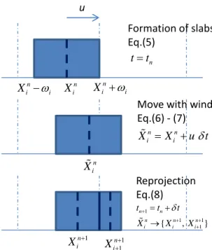
Figure 1.Advection step of the scheme of Michael Galperin.
mass in the cell Mi and the position of the centre of mass
Xi,Xi∈ [xi−0.5, xi+0.5]:
Mi = xi+R0.5
xi−0.5
ϕ(x)dx,
Xi =M1
i
xi+R0.5
xi−0.5
xϕ(x)dx.
(4)
Let us represent the mass distribution in each grid cell via the rectangular slab:
πin(x)=
1 2ωni,
x−Xin≤ωni
0, otherwise
, (5)
where n is the time step and ωni=
min Xni −xi−0.5
,Xin−xi+0.5
is the distance from the centre of mass Xin to the nearest border of the cell i. Equation (5) defines the widest unit-volume slab that can be confined inside the cell (Fig. 1) for the given centre of mass. The advection scheme consists of a transport step and a re-projection step. At the transport step, each slabπi is moved along the velocity fieldu(x). Advection of the slab does not change its shape within the time stepδt=tn+1−tn, but can
move it anywhere over the domain or bring it outside. In essence, the slab transport is replaced with advection of its mass centre, which during this time step becomes analogous to a Lagrangian particle:
Xni+1=Xin+
tZn+1
tn
u(Xni, t )dt, (6)
whereu(Xni, t )is the wind speed at the mass centre location. The original Galperin scheme employed wind at the cell mid-pointxi and used explicit first-order time discretisation:
u(xin, tn)=uni. Then the transported slab is given by
eπin(x)=πin(x−uniδt ). (7)
Following the transport step (7), the massesMk and cen-tres of massXkof the receiving set of cellsk∈Kare updated using the transported slabseπin:
Mkn+1=
Nk P
i=1
αi,kMin,
Xkn+1= 1
Mkn+1 Nk P
i=1
βi,kMin,
(8)
whereαi,k= Rxk+0.5
xk−0.5eπ
n
i(x)dx and βi,k= Rxk+0.5
xk−0.5xeπ
n i (x)dx correspond to the mass and the first-moment fractions arriv-ing from the celliinto cellk. The integrals are easy to eval-uate due to the simple form ofπin(x)in Eq. (5). In essence, Eq. (8) describes a mass-conservative projection of the ad-vected slab to the computation grid.
The coefficients αi,0=R−∞0.5eπin(x)dx and αi,I+1=
R∞
I+0.5eπ
n
i(x)dx determine the transport outside the domain through the left and right borders, respectively; that is, the scheme is fully accountable and mass-conservative sinceP
k
αi,k=
∞ R
−∞e
πin(x)dx=1 for each i. Also, since the functions πin(x) are nonnegative, the coefficients αi,k are nonnegative, and consequentlyMkn+1≥0 as long asMin≥0 for alli. It means that the scheme is positively defined for any simulation set-up:u, 1t,and discretisation grid.
In multiple dimensions, the slabs are described by the to-tal mass in multidimensional cells and centres of mass along each dimension. In two dimensions, an analogue of Eq. (5) will be
5ni,j(x, y)=πi,jn (x)πi,jn (y), (9) where the functionsπi,j(x)andπi,j(y)depend onXi,j and
Yi,j, respectively. The advection step in the form of Eq. (7) and the slab projection integrals Eq. (8) are then defined in 2-D space.
However, a simpler procedure used in the original scheme is obtained with dimensional splitting, where the transport in each dimension is processed sequentially with the grid pro-jection applied in between. For anx−ysplit, the intermediate distribution for each rowj is obtained by setting
5ni,j+1/2(x, y)=eπi,jn (x)πi,jn (y), (10) evaluating αi,k and βi,k from eπi,jn (x) and updating
Mi,j, Xi,j and Yi,j. Since
Ryj+0.5
yj−0.5πi,j(y)dy=1 and Ryj+0.5
yj−0.5yπi,j(y)dy=Y
n
Theyadvection is then performed by taking the transport step forπi,jn+1/2(y)starting fromYin+1/2, evaluatingαi,kand
βi,kfromeπn
+1/2
i,j (y), and applying the re-projection Eq. (11) withX andY inverted. The generalisation to three dimen-sions is analogous.
2.3 Relation of the Galperin scheme to other approaches
The Galperin scheme shares some features with other ap-proaches (see the reviews of Rood, 1987, and Lauritzen et al., 2011). Arguably the closest existing scheme is the finite-volume approach of Egan and Mahoney (1972), hereinafter referred to as EM72, and Prather (1986), hereinafter P86. The main similarity between these schemes is the represen-tation of the mass distribution as a set of slabs (rectangular in EM72 and continuous polynomial distributions in P86), one per grid cell, with the mass centre identified via the slab first moment, plus additional constraints. During the EM72 and P86 advection steps, mass and the first moment are con-served, similarly to the reprojection step (8). However, the similarity ends here.
There are several principal differences between the EM72/P86 and Galperin algorithms.
Firstly, in EM72 the slab width is computed via the second moment (variance) of the mass distribution in the grid cell. P86 uses the second moments to constrain the shape of the polynomials. As a result, this moment has to be computed and stored for the whole grid, and the corresponding conser-vation equation has to be added, on top of those for the mass and the first moment. Galperin’s approach does not require the second moment, instead positioning the slab against the cell wall. In fact, EM72 pointed out that the second moment can be omitted, but did not use the wall-based constraint in such a “degenerated” scheme, which severely affected its ac-curacy.
Secondly, EM72 uses the movements of the slabs in ad-jacent grid cells to calculate the mass flows across the bor-der. Such local consideration requires the Courant number to be less than 1: the so-called “portioning parameter” (a close analogy to the Courant number in the scheme) is lim-ited between 0 and 1. The same limitation is valid for the P86 approach. Galperin’s scheme can be applied at any Courant number and its re-projection step can rather be related to Lin and Rood (1996).
– Real-wind tests have shown that the scheme has difficul-ties in complex-wind and complex-terrain conditions, similar to EM72 (Ghods et al. 2000).
– The explicit forward-in-time advection (Eq. 7) is inac-curate.
– The scheme, being very good with individual sharp plumes over zero background, noticeably distorts the smoother fields with a non-zero background – see P08. In addition, the accuracy of the dimension split was increased via symmetrisation: the order of dimensions in SILAM rou-tines is inverted each time step:x−y−z−z−y−x(Marchuk, 1995).
3.1 Lateral and top boundary conditions
The open boundary for the outgoing masses is kept in SILAM regional simulations. The inflow into a limited-area domain is defined via prescribed concentration at the bound-ary (Eq. 3),α=0,β=1,γ =ϕl. The mass coming into the domain during a single time step is equal to
M1in=ϕl(x0.5) u(x0.5)ℵ(u(x0.5))δt,
MIin=ϕl(xI+0.5)|u(xI+0.5)| ℵ(−u(xI+0.5))δt.
(12) Hereℵ(u) is a Heaviside function (=1 if u >0, =0 if
u≤0). Assuming the locally constant wind, we find that
Min is distributed uniformly inside the slab, similar to that of Eq. (5). For e.g. the left-hand border, the continuous form will read
5nin+1(x)=
ϕ
l(x0.5)ℵ(u(x0.5, tk))δt, x∈x0.5, x0.5+u(x0.5, tn)ℵ(u(x0.5, tn)) δt
0, otherwise .
(13) It is then projected to the calculation grid following Eq. (8).
The top boundary follows the same rules as the lateral boundaries. At the surface, the vertical wind component is zero, which is equivalent to closure of the domain with re-gard to advection.
Global-domain calculations require certain care: SILAM operates in longitude–latitude grids; that is, it has singular-ity points at the poles and a cut along the 180◦E line. For longitude, if a position of a slab part appears to be west of
360◦, respectively. Resolving the pole singularity is done by reserving a cylindrical reservoir over each pole. The radius of the reservoirs depends on the calculation grid resolution but is kept close to 2◦. The calculation grid reaches the borders of the reservoirs, whose mean concentrations are used for the lateral boundary conditions:
ϕy2=y2_0.5 =ϕS_pole(t, z); ϕy2=y2_J+0.5 =ϕN_pole(t, z).
(14) Vertical motion in the pole cylinders is calculated sepa-rately using the vertical wind component diagnosed from the global non-divergence requirement.
3.2 Extension of the scheme for complex wind patterns The original Galperin scheme tends to accumulate mass at stagnation points where one of the wind components is small. Similar problems were reported by Ghods et al. (2000) for the EM72. Ghods et al. (2000) also suggested an explanation and a generic principle for solving the problem: increasing the number of points at which the wind is evaluated inside the grid cell. For application in the Galperin scheme, it can be achieved by separate advection of each slab edge instead of advecting the slab as a whole. This allows for shrinking and stretching of the slab following the gradient of the velocity field. Formally, this can be written as follows.
Let us again consider the 1-D slab that has been formed according to Eq. (5). Its edges are
XL, i=Xi−ωi, XR,i=Xi+ωi. (15) The advection step takes the wind velocity at the left and right slab edges and transports them in a way similar to Eq. (6) with the corresponding wind velocities. The new slab is formed as a uniform distribution between the new positions of the edges:
e
πik+1(x)=
1
e
XkR,i−eXL ,ik , Xe k+1
L,i ≤x≤Xe k+1
R,i
0, otherwise
, (16)
whereXekL,i,XeR,ik are the new positions of the slab edges at the end of the time step. This new slab is then projected fol-lowing Eq. (8).
3.3 Changing wind along the mass-centre trajectory The explicit advection step (Eq. 7) is inaccurate and can be improved under the assumption of linear change of wind in-side each grid cell, with values at the borders coming from the meteo input:
u(x)=u(xi−0.5, tn)
(xi+0.5−x)
(xi+0.5−xi−0.5)
+u(xi+0.5, tn)
(x−xi−0.5)
(xi+0.5−xi−0.5)
xi−0.5≤x≤xi+0.5. (17)
Then, the trajectory equation (6) can be piece-wise inte-grated analytically for each slab edge. Let us denote1u=
ui+0.5−ui−0.5, 1t=tn+1−tn, α=1u/1t and consider the transport starting at e.g.xi−0.5. Then, the time needed for
passing through the entire cell,1x=xi+0.5−xi−0.5, is
Tcell=log(1+α 1x ui)/α. (18)
If1t < Tcell, the point will not pass through the whole cell
and stop at
x1t =xi−0.5+ui(expαt −1)/α. (19) Applying sequentially Eqs. (18) and (19) until completing the model time step1t, one obtains the analytical solution for the final position of the slab edges.
This approach neglects the change of wind with time. However, the integration method is robust, since the linearly interpolated wind field is Lipschitz-continuous everywhere, which in turn guarantees the uniqueness of the trajectories of
XLandXR. Therefore, using the analytic solution Eqs. (18) and (19), the borders of the slabs will never cross.
3.4 Reducing the shape distortions
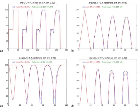
The original scheme tends to artificially sharpen the plume edges and to gradually redistribute the background mass in the vicinity of the plume towards it (Fig. 2, blue shapes). Similar “antidiffusive” distortions were also reported by P08 and by EM72 – for their scheme.
The reason for the feature can be seen from Eq. (8): if a large mass is concentrated at one of the grid cell sides, the centre of mass becomes insensitive to the low-mass part of the cell; that is, a small mass that appears there from the neighbouring cell is just added to the big slab with little effect on its position and width.
A cheap, albeit not rigorous, way to confront the effect is to compensate for it via an additional small pull of the mass centre towards the cell mid-point before forming the slab for advection:
ˆ
Xni =xi+(Xin−xi)(1−ε), (20) whereεis the smoothing factor. The adjusted mass centreXˆni
is then used to form the slab Eq. (5).
a) b)
c) d)
Figure 2.Shape preservation tests:(a)step,(b)triangle peak,(c)sine-shaped dip, and(d)sine-shaped peak. Sequential positions are shown: “r” denotes the scheme without a smoother, “r_diff” with it. The legend includes the number of times steps made. Wind is from left to right; Courant=0.4.
ε∼0.08 (Fig. 2, red shapes). This behaviour and the value were similar for various Courant numbers and tests. It is also seen from the spectral features of the scheme in the next sec-tion – and further discussed in relasec-tion to scheme tests. 3.5 Analysis in frequency space
The non-linearity introduced by the coupling of cell mass and centre of mass in Eq. (8) makes formal stability and conver-gence analysis after Charney et al. (1950) difficult. However, the features of the scheme can be investigated numerically following the approach of Kaas and Nielsen (2010).
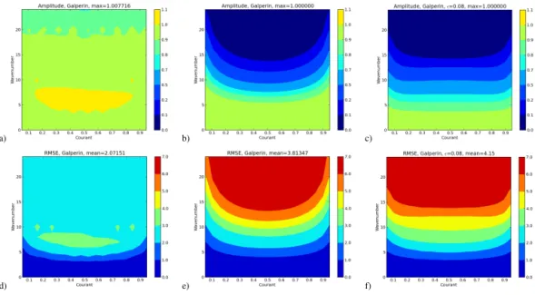
The scheme was run for 200 time steps in a 1-D domain with 100 grid points. For each wave number up to 25, the scheme was initialised with the corresponding sine function and run with Courant numbers ranging from 0.05 to 0.95 in steps of 0.05. This allowed evaluation of the spectrally re-solved root mean squared error (RMSE) and, after a Fourier transform, the spectral amplification factor (cumulative for the 200 steps) for each wave number. The amplification fac-tor quantifies the scheme’s ability to resolve the correspond-ing harmonics, while the RMSE additionally includes the ef-fect of phase errors and possible spurious modes. Since the scheme is formulated for nonnegative concentrations, a con-stant backgroundB=1 is added to each waveform.
Figure 3 presents the amplification factor and RMSE for the Galperin scheme without the smoother (panels a, d) and with it,ε=0.08 (panels c, f). Furthermore, the impact of doubling the background component to twice the wave am-plitude is shown (panels b, e). In the case of B=1, the scheme without the smoother shows only minor damping of all considered wave numbers (kup to 25). The RMSE has a maximum forkof between 5 and 10 but stays almost con-stant fromk=10 tok=25. This shows the scheme’s ability to resolve sharp gradients when there is no significant back-ground. The cumulative amplifying factors for some wave-lengths exceed 1, but this does not imply instability, since the single-step amplifying factors fluctuate depending on the po-sitions of the centres of mass. If the integration is continued over a large number of time steps (not shown), the solution converges to a combination of rectangular pulses (a similar feature was mentioned in EM72 for that scheme).
a) b) c)
d) e) f)
Figure 3.Spectral analysis for 1-D. Panels(a)and(d): amplification factor (AF) and RMSE, respectively, for the Galperin scheme without a smoother;(b),(e): AF and RMS for the Galperin scheme with a large background;(c),(f): AF and RMSE for the Galperin scheme with smootherε=0.08.
Eq. 8), which leads to a similar damping of the higher fre-quencies as in Fig. 3c, f.
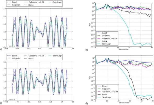
To further investigate the spectral response of the scheme, it was evaluated with a broadband input:
f (x)=sin(2π xcos(20π x))+B. (21) Figure 4, right panel, depicts the power spectral densities for the exact and numerical solutions after a single revolution with CF=0.7 and 100 grid points. The corresponding solu-tions are shown in the leftpanel. For the comparison, results are also shown for the fourth-order Bott (1989) scheme with-out shape preservation, and for a generic non-conservative upstream semi-Lagrangian scheme with cubic spline inter-polation.
With B=1, all schemes capture the first spectral peaks aroundk=10 and therefore resolve most of the spectral con-tent. Without a smoother, the Galperin scheme that follows the spectrum of the true solution also resolves the spectral features aroundk=30. Application of the smoother leads to a damping effect throughout the spectrum, including the spu-rious high-frequency components, such as the peak atk=40. This illustrates the use of the smoother for reducing over- and under-shoots, as discussed in Sect. 3.4.
Similarly to the single-harmonic tests, the situation changes in the presence of a significant background (B=2). Regardless of smoothing, the Galperin scheme damps the spectral peaks starting aroundk=10, which corresponds to the reduction of amplitude visible in the numerical solution.
4 Connection of the advection scheme with other SILAM modules
Construction of the dispersion model using the Galperin ad-vection scheme as its transport core is not trivial because all other modules should support the use of the sub-grid infor-mation on positions of the mass centres. In some cases it is straightforward, but in others one can only make the module to return them undamaged back to advection.
4.1 Vertical axis: combined advection, diffusion, and dry deposition
For the vertical axis, SILAM combines the Galperin advec-tion with the vertical diffusion algorithm following the ex-tended resistance analogy (Sofiev, 2002), which considers the air column as a sequence of thick layers. Vertical slabs within these layers are controlled by the same 1-D advection, which is performed in absolute coordinates – either z- or p-, de-pending on the vertical (height above the surface or hybrid). Settling of particles is included in advection for all layers ex-cept for the first one, where the exchange with the surface is treated by the dry deposition scheme.
The centres of masses are used but not modified by dif-fusion: the effective diffusion coefficient between the neigh-bouring thick layers is taken as an inverse of aerodynamic re-sistance between the centres of mass of these layers (Sofiev, 2002):
< Ki,i+1>=
1zi,i+1
ZRi+1
Zi
dz Kz(z)
a) b)
c) d)
Figure 4.Example of input and output spectra for broadband input to the advection schemes with zero and nonzero background levels. Left panels: exact and numerical solutions. Right panels: power spectrum densities initially and after one revolution. Top:B=0; bottom: B=1.0.
The effective thickness1zi,i+1is taken to be proportional
to the pressure drop between the centres of masses, which ensures equilibration of mixing ratios due to diffusion.
In the lowest layer, the dry deposition velocity is calcu-lated at the height of the centre of mass Z1 following the
approach of Kouznetsov and Sofiev (2012).
The advantages of using the mass centres as the vertical diffusion meshes are discussed in detail by Sofiev (2002), where it is shown that the effect can be substantial if an in-version layer appears inside the thick dispersion layer. Then the location of the mass centre above/below the inversion can change the up/down diffusion fluxes by a factor of several times.
4.2 Emission-to-dispersion interface
Emission data are the only source of sub-grid information apart from the advection itself: location of the sources is transformed into the mass centre positions of their emission. For point sources, the mass is added to the corresponding grid cell and centres of masses are updated:
ˆ
Mij k=Mij k+Mems ˆ
Xij k=(Xij kMij k+MemsXems)/Mˆij k
ˆ
Yij k=(Yij kMij k+MemsYems)/Mˆij k
ˆ
Zij kk =(Zij kk Mij k+MemsZkems)/Mˆij k
, (23)
whereMemsis the mass emitted to the cell(i, j, k)during the
time step,Xems, Yemsare the coordinates of the source in the
grid andZemsk is the effective injection height in the layerk, equal to the middle of the layer if no particular information is available.
For area sources, the approach depends on the source grid. If it is the same as the computational one, the mass centre is put to the middle of the cell (no extra information can be obtained). If the grids are different, the source is re-projected. For each computational grid cell(i, j ),the centre of mass of emission is
Xem,ij= RR
(x,y)∈(i,j )
xM(x, y)dxdy RR
(x,y)∈(i,j )
M(x, y)dxdy , (24)
Yem,ij= RR
(x,y)∈(i,j )
yM(x, y)dxdy RR
(x,y)∈(i,j )
M(x, y)dxdy ,
whereM(x, y)denotes the original source distribution. After that, the procedure is the same as in the case of point source Eq. (23).
4.3 Meteo-to-dispersion interface
(unless they are directly available from the input data). More-over, the pre-processor needs to ensure consistency between the flow and air density fields (Prather et al. 1987; Rotman et al., 2004; Robertson and Langner, 1999). This is particularly important with the present advection scheme, since mixing ratio perturbations caused by the mass-flow inconsistency are not suppressed by numerical diffusion.
The wind pre-processing follows the idea of a “pressure fixer”, which means adding a correction δV to the original horizontal wind fieldV0such that for their sum, the vertical integral of mass flux divergence corresponds to the surface pressure tendency:
Z ps
0
∇ ·(V0+δV)dp= −∂ps
∂t , (25)
where the surface pressure tendency ∂ps/∂t is evaluated
from the meteorological input data. The correctionδV is not uniquely determined, and SILAM adopts the algorithm of Heimann and Keeling (1989), where the correction term is given by the gradient of a 2-D potential function:
δV= ∇ψ (x, y). (26)
Substituting Eq. (26) into (25) yields a Poisson equation forψ (x, y), which is solved to subsequently recoverδV. The obtained correction flux is then distributed within the column proportionally to the air mass in each layer, ending up with the corrections to the horizontal winds. The vertical wind is then evaluated in each column to enforce the proper air-mass change in each cell.
4.4 Chemical module interface
This interface is implemented in a very simple manner: the mass centres are not affected by the transformations. The chemical module deals exclusively with concentrations in the grid cells. The newly created mass is added to the existing one, thus accepting its centre position in the cell. If some species did not exist before the transformation, the new mass centre is put to the middle point of the cell.
5 Testing the Galperin advection algorithm 5.1 Standard tests
A set of basic tests and comparison with some classical ap-proaches has been presented by Galperin (1999) and P08 for the original scheme, along with Bott, Holmgren, and several other schemes. Their main conclusions were that the scheme is very good for sharp-edge patterns: in particular, it trans-ports delta functions without any distortions. It had, however, issues with long slopes, smooth shapes, etc., where the ten-dency to gradually convert them to a collection of rectangles was noticeable.
Figure 5.Linear-motion tests with a constant-release point source at Xsand varying wind speed along thexaxis. Upper panel: Courant
number; lower panel: concentration (arbitrary unit). Wind blows from left to right. Without smoother.
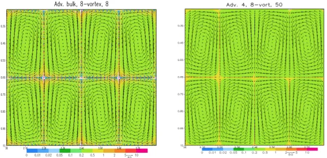
Addressing these concerns, tests used during the scheme improvements and implementation in SILAM included puff-over-background, conical and sine-shaped peaks and dips, etc. (some examples are shown in Fig. 2), a divergent 1-D high-Courant wind test in the 1-1-D divergent wind field (Fig. 5), a constant-level background field in eight vortices with stagnation points (Fig. 6), and rotation tests for various shapes (Fig. 7).
The scheme stays stable at arbitrarily high Courant num-bers and handles the convergence and divergence of the flows (Fig. 5).
Transport and rotation tests of the improved scheme main-tain low distortions of the shapes: the L2 norm of the
er-ror varies from 0.1 % up to 3.8 % of the initial-shape norm – for the most challenging task in Fig. 7. The effect of the improvements in comparison with the original scheme is demonstrated in Fig. 2, where the blue contours show the results of the original scheme. In particular, application of the smoothing Eq. (20) reduced the distortions of smooth shapes (red curves), largely resolving the concerns of P08: Fig. 2b presents the same test as one of the P08 exercises. However, the smoother also leads to a certain numerical vis-cosity of the scheme, so its use in problems requiring non-diffusive schemes (e.g. narrow plumes from accidental re-leases) should be avoided.
Figure 6.Test with eight non-divergent 2-D vortices. Left panel: test of the original scheme (5)–(7), time step 8; right panel: improved scheme (15)–(16), time step 50. Both tasks were initialised with constant value 0.4, also used as boundary conditions. Without smoother.
5.2 Global 2-D tests
Performance of Galperin’s advection scheme in the global spherical domain was assessed with the collection of manding tests of Lauritzen et al. (2012). The cases are de-signed to evaluate the accuracy of transport schemes at a wide range of resolutions and Courant numbers. The tests used a prescribed non-divergent 2-D velocity field defined on a sphere and consisting of deformation and rotation, so that the initial concentration pattern is reconstructed at the end of the test, t=T, providing the exact solution ϕ(t=0)=
ϕ(t=T ).
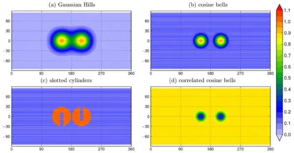
Four initial concentration distributions were used (Fig. 8): “Gaussian hills” with unity maximum value, “cosine bells” with a background of 0.1 and maxima of 1, “slotted cylin-ders” – a rough pattern with a 0.1 background and 1 max-imum level, and “correlated cosine bells” – the distribution obtained from “cosine bells” with a function
ϕccb=0.9−0.8ϕ2cb. (27)
The tests were run with SILAM on a global regular non-rotated lon–lat grid, withR=6400 km andT =12 h. Spatial resolutions were 6, 3, 1.5, 0.75, 0.375, and 0.1875◦, each run with mean Courant numbers of ∼5.12,∼2.56, and∼0.85 (for a 6◦ grid they correspond to the model time step of
T /12=1 h,T /24=30 min, andT /72=5 min), and a total of 18 runs for each initial pattern.
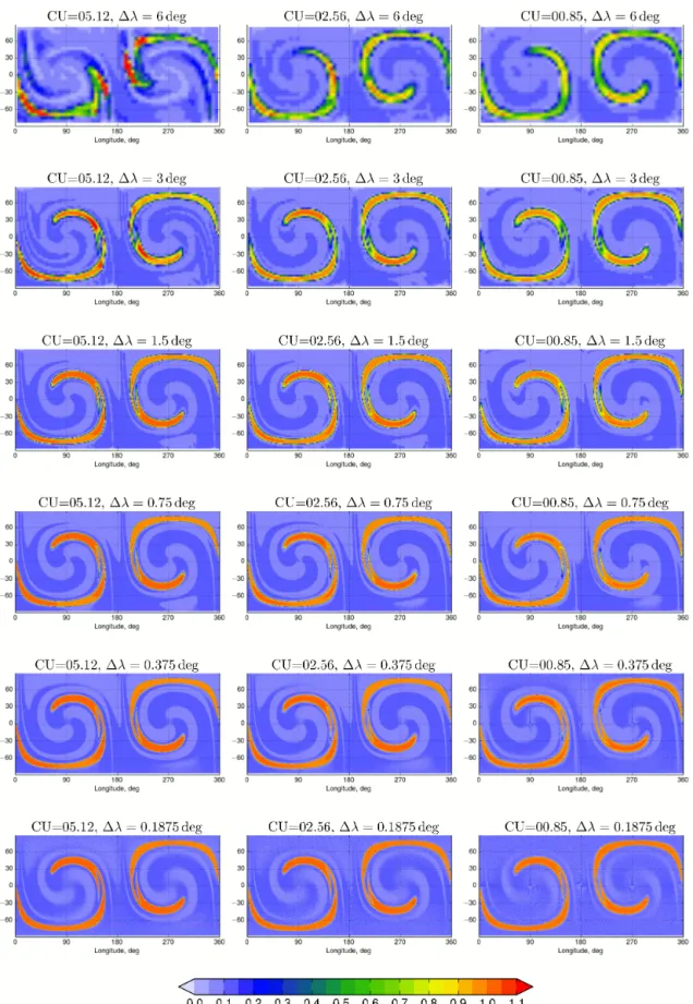
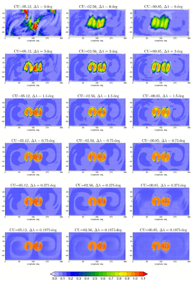
Examples of the most challenging runs with slotted cylin-ders at t=T /2 and att=T are shown in Figs. 9 and 10, respectively. The corresponding error fields are collected in Fig. 11 as decimal logarithms of the absolute difference be-tween the corresponding field in Fig. 10 and the slotted-cylinder initial shape of Fig. 8. The main complexity of the
test was in reproducing the very tiny sharp-edge structures obtained from the cylinder cut att=T /2 – and then return-ing them back byt=T. The pictures, together with the error field att=T (Fig. 11), show that already 24 time steps al-low the scheme to make the shape recognisable (3◦,C=5.12 pattern), whereas 48 time steps allow for the main details to show up. Expectedly, certain deviations at the cylinder edge remain at any resolution – as is visible from the error fields.
Deviation of the resulting field ϕT =ϕ(t=T ) from the initial shapeϕ0=ϕ(t=0)was considered in three spaces:
L2,L∞, andL1. The corresponding distance metrics are
de-fined as follows:
l2=
"
S[(ϕT −ϕ0)2]
S[ϕ02]
#1/2
, l∞=max|ϕT−ϕ0|
maxϕ0
,
l1=
S[|ϕT−ϕ0|]
S[|ϕ0|]
, (28)
whereS[•] is an area-weighted sum over latitude and longi-tude. The values of these three metrics for all model runs are presented in Fig. 12. The main interest of these curves is that they show the rate of the scheme convergence (straight grey lines correspond to the first- and second-order convergence rates). Expectedly, the rates depend on the transported shape (the smoother the shape, the faster the convergence) and on the norm used. Thus, the scheme converges inL1faster than
in L2, whereas inL∞ no convergence in the case of sharp
edges is an expected result. The rate in theL2norm is in
be-tween the first and the second order, whereas inL1it is close
to the latter one.
0 0.05 0.1 0.15 0.2 0.25 0.3 0.35 0.4 0.45
0 0.1 0.2 0.3 0.4 0.5 0.6 0.7 0.8
0 0.05 0.1 0.15 0.2 0.25 0.3 0.35 0.4 0.45 0.5
Figure 7.Double-vortex rotation tests for a rectangular split between the vortices (upper panels); three single-cell peaks and two connected rectangles (middle panels); and sin- and cone-shaped surfaces (lower panels). A series of time steps is shown in the left panels, except for the low panel (shownt=361). Right panels: error field after one full revolution (obs 10-fold more sensitive scale and relativeL2norm given
Figure 8.Initial shapes of the puffs for the 2-D global test on the sphere.
Since these initial patterns are related by Eq. (27), the con-centration fields during the tests should maintain the same relation. The scatter plots of the concentrations in these two tests give an indication of how the ratio is kept. Ideal advec-tion would keep all points on a line given by Eq. (28). The results of the tests fort=T /2 are shown in Fig. 13, where the results with and without the smoother in Eq. (20) are pre-sented. The smoother improves the scheme mixing preserva-tion; that is, it can be recommended to chemical composi-tion computacomposi-tions, which usually also tolerate some numeri-cal viscosity.
5.3 Global 3-D test with real wind
Testing the scheme with real-wind conditions has one ma-jor difficulty: there is no accurate solution that can be used as a reference. An exception is simulations of the constant-mixing-ratio 3-D field, which, once initialised, must stay constant throughout the run. Deviation from this constant is then the measure of the model quality. Such a test verifies both the scheme and the meteo-to-dispersion interface, which has to provide the consistent wind fields.
The constant-vmr test was set with winds taken from the ERA-Interim archive of ECMWF, for the arbitrarily selected month of January 1991 (Fig. 15). The model was initialised with vmr=1 and run with 3◦of lon–lat resolution and a time step of 30 min (max Courant number exceeding 13 in the stratosphere and reaching up to 2–3 in the troposphere). The model top was closed at 10 Pa, which corresponds to the top level of the ERA-Interim fields. The procedure described in Sect. 4.3 was used to diagnose the vertical wind component. The results of the test are shown in Fig. 15, which depicts the model state after 240 h of the run, panel a) showing the boundary-layer vmr, and panel b) presenting it in the
strato-sphere. The zonally averaged vertical cross section is shown in panel c). Green colours in the pictures correspond to less than 1 % of the instant-field error.
An important message is that the limited distortions about 1–2 % are visible in a few places, but they are not related to topography, rather being associated with the frontal zones and cyclones. The comparatively coarse spatial and tempo-ral resolution of the test makes the associated changes of the wind quite sharp, so that the dimension-split errors start manifesting themselves. Smoother flows in the stratosphere posed minor challenges for the scheme. The L2 error (not shown) is approximately proportional to the model time step.
6 Discussion
0.001 0.01 0.1 1 0.19 0.38 0.75 1.5 3 6 CU=0.85 CU=2.56 CU=5.12 0.001 0.01 0.1 1 0.19 0.38 0.75 1.5 3 6
l2 Slotted cylinder
CU=0.85 CU=2.56 CU=5.12 0.001 0.01 0.1 1 0.19 0.38 0.75 1.5 3 6
l2 Cosine holes
CU=0.85 CU=2.56 CU=5.12 0.001 0.01 0.1 1 0.19 0.38 0.75 1.5 3 6 CU=0.85 CU=2.56 CU=5.12 0.001 0.01 0.1 1 0.19 0.38 0.75 1.5 3 6
l1 Slotted cylinder
CU=0.85 CU=2.56 CU=5.12 0.001 0.01 0.1 1 0.19 0.38 0.75 1.5 3 6
l1 Cosine holes
CU=0.85 CU=2.56 CU=5.12 0.001 0.01 0.1 1 0.19 0.38 0.75 1.5 3 6 ∞ CU=0.85 CU=2.56 CU=5.12 0.001 0.01 0.1 1 0.19 0.38 0.75 1.5 3 6
l∞ Slotted cylinder
CU=0.85 CU=2.56 CU=5.12 0.001 0.01 0.1 1 0.19 0.38 0.75 1.5 3 6
l∞ Cosine holes
CU=0.85 CU=2.56 CU=5.12
Figure 12.Dependence of the performance metrics l1, l2, andl∞for the spherical 2-D tests with initial shapes of Fig. 8. Dashed straight lines mark the slope for the first and second order of convergence. Without smoother.
transformation calculations. At present, the actual SILAM applications are performed with Courant close to but mostly smaller than 1 to avoid such problems.
The above challenges are mostly technical and their solu-tion allows the scheme to demonstrate strong performance with low computational costs.
In particular, by attributing the release from point source to its actual location, one can reduce the impact of the common problem of Eulerian models: point release is immediately di-luted over the model grid cell. This substantially improves the transport but does not solve the problem completely: (i) the chemical module still receives the diluted plume con-centration, and (ii) the slab size in the case of the source near the centre of the grid cell will still be as large as the grid cell itself. A more accurate solution would be the
plume-in-grid or similar approaches, which is being built in SILAM. Another example of the sub-grid information usage is utili-sation of full meteorological vertical resolution to calculate effective values of meteo variables for thick dispersion layers (Sofiev, 2002).
CU=05.12, ∆λ= 0.75 deg CU=02.56, ∆λ= 0.75 deg CU=00.85, ∆λ= 0.75 deg
CU=05.12, ∆λ= 0.375 deg CU=02.56, ∆λ= 0.375 deg CU=00.85, ∆λ= 0.375 deg
CU=05.12, ∆λ= 0.1875 deg CU=02.56, ∆λ= 0.1875 deg CU=00.85, ∆λ= 0.1875 deg
Figure 13.Mixing preservation test for cosine bells and correlated cosine bells Eq. (27) att=T /2. Every two lines show the tests without (upper line) and with (lower line) a smoother (20).
SILAM heavily relies on such features of Galperin scheme as mass conservation and accountability: the scheme pro-vides complete mass budget including transport across the domain boundaries. In particular, nesting of the calculations is straightforward and does not need the relaxation buffer at
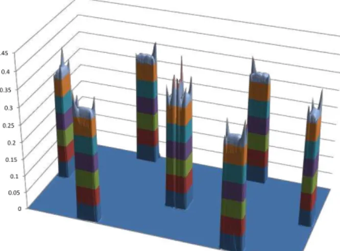
Figure 14.A histogram of the mixing diagnostic (stacked) for the same resolutions, Courant number and smoother factor as in Fig. 13. Metrics are the following (see text and Lauritzen et al. (2012) for more details):lr is “real mixing”,luis “range-preserving
unmix-ing”, andlois “overshooting”. Values are relative to the reference
CSLAM performance in L14 tests. The picture is comparable with panel(b)of Fig. 15 in L14.
still possible (Fig. 2), which can be reduced by the smoother described in Sect. 3.4, Eq. (20).
6.1 Standard advection tests
Evaluating the Galperin scheme with the simple tests (Figs. 2–7), one can point out the known issues of the classi-cal schemes resolved in the Galperin approach: high-order algorithms suffer from numerical diffusion, oscillations at sharp gradients (require special efforts for limiting their am-plitude), high computational costs and stringent limits to Courant number. None of these affects the Galperin scheme. The main issue noticed during the implementation of the original scheme was the unrealistically high concentrations near the wind stagnation points. Thus, the concentration pat-tern at the test Fig. 6a resembles the situation of a divergent wind field. However, it is not the case: the 2-D wind pattern is strictly solenoidal. The actual reason is insufficient reso-lution of the advection grid: one centre of mass point is not enough if the spatial scale of the wind variation is compa-rable with the grid cell size. Tracking the edges of the slab rather than its centre resolves the problem (Fig. 6b).
The other challenging tasks for Galperin algorithm were those with smooth background and soft gradients, a frequent issue for semi-Lagrangian schemes, which is easily handled by more diffusive approaches. This feature was visible in the P08 tests where the scheme noticeably distorts the Gaussian and conical plumes. For the puff-over-background pattern, the scheme makes a single low-mass dip in the vicinity of the puff, which receives this mass (Fig. 2). From a formal point of view, the scheme does not conserve the higher
mo-a)
b)
c)
Figure 15. Constant-vmr test with real-wind conditions after
122 h. (a) vmr within the boundary layer, (b) vmr above the
tropopause, and (c) zone-average vertical cross section of vmr. Without smoother.
6.2 Global 2-D and real-wind advection tests
The application of the scheme to the highly challenging tests of Lauritzen et al. (2012) allowed its evaluation in a global 2-D case and comparison with the state-of-the-art schemes evaluated by L14 and Kaas et al. (2013).
Performing these tests with different spatial and temporal resolutions, as well as Courant numbers, suggested that the scheme has an “optimal” Courant number for each spatial resolution where the error metrics reach their minimum, so that the increase in temporal resolution is not beneficial. In-deed, in Fig. 12 the low Courant runs are by no means the most accurate. This is not surprising: for an ideal scheme, increasing the grid resolution and reducing the time step should both lead to gradual convergence of the algorithm; that is, the error metrics should reduce. For real schemes, higher temporal resolution competes with accumulation of the scheme errors with increasing number of steps. Conver-gence in L14 tests was still solid for all fixed Courant num-ber series (Fig. 12), but excessive temporal resolution (spe-cific to each particular grid cell size) was penalised by higher errors. Similarly, the most accurate representation of the cor-related patterns is obtained from the runs with the intermedi-ate Courant numbers (Fig. 13). This seems to be a common feature: the same behaviour was noticed by L14 for several schemes.
High optimal Courant numbers, however, should be taken with care. For L14, the smooth wind fields reduced the dimension-split error and made the long time steps partic-ularly beneficial.
It is also seen (Fig. 11) that the best performance, in case of a near-optimal Courant, is demonstrated by the high-spatial-resolution simulations, which have reproduced both the sharp edges of the slotted cylinders, the flat background and the cylinder’s top planes.
The scheme demonstrated a convergence rate higher than 1 for all metrics and all tests with smooth initial patterns. Even for the most stringent test with the slotted cylinders, the scheme showed the first-order convergence rate in theL1
norm (Fig. 12).
Among the other features of the solution, one can notice a certain inhomogeneity of the background field away from the transported bodies. The error is very small (<10−4)for high-resolution cases (Fig. 11) and <0.1 % for inexpensive set-ups, such as1λ=0.75,C=2.56. For coarser resolutions, it grows. The inhomogeneity also grows with Courant num-ber, which is opposite to the decreasing error of representa-tion of the shapes themselves. The issue originates from the dimension-split error in polar areas, where the spatial scale of wind change becomes comparable with the distance passed by the slabs within one time step.
Similar non-monotonicity of background is visible for some schemes tested by L14. Unfortunately, no error fields are given there, but Figs. 7–10 there are comparable with our Fig. 9 (results without a smoother). With few
excep-tions (schemes TTS-I and LPM, notaexcep-tions of L14), all algo-rithms manifested such patterns unless filters are applied. For some schemes (SFF-CSLAM3, SFF-CSLAM4, UCISOM-CS, CLAW, and CAM), these inhomogeneities are visible also for the tests with shape-preserving filters. One should note however that the 0.1 level, which distinguishes between the two violet colours in Figs. 9 and 7–10 of L14, corre-sponds to the background level in the slotted-cylinder test. As a result, even a very small deviation leads to the appearance of such shapes in the plots (note the stripes in the background of Fig. 8).
Comparing the so-called “minimal resolution” threshold forL2, the norm of cosine bells to reach 0.033 (Fig. 3 of L14)
for SILAM was about 0.75◦, which puts it in the middle of that multi-model chart (the specific place depends on whether the shape preservation is considered or not).
Another criterion can be the optimal convergence ofL2
andL∞norms for Gaussian hills: about 1.7–1.8 for SILAM – this is again in the middle of the L14 histograms, in the second half if the unlimited schemes (without shape-preservation filters) are considered and in the first half if the unphysical negative concentrations are suppressed (since the Galperin advection is strictly positively defined, no extra ef-forts are needed to satisfy this requirement).
Interestingly, the L14 tests were limited with 3◦ as the coarsest resolution, and it was pointed out that the schemes start converging only when a certain limit, specific to each scheme, is reached. The SILAM results show similar be-haviour only for the lowest Courant number (red lines in Fig. 12), which indeed required appropriate resolution to start working. Higher Courant set-ups were much less restrictive (the errors decrease with growing resolution also for coarse grids) and, as already pointed out, often worked better than the low Courant runs (similar to many L14 schemes).
The scheme demonstrated limited distortion of pre-existing functional dependence – see the cosine bells and correlated cosine bells tests in Eq. (27) (Fig. 13). Formal scores suggested by Lauritzen et al. (2012) calculated for the Galperin scheme are shown in Fig. 14. Notations are the fol-lowing.lo, “overshooting”, describes the values that fell
out-side the rectangular [0.1:1] (Fig. 13),lu, “shape-preserving
unmix”, describes the values inside that rectangular but out-side the “lens” formed by its diagonal (0.1, 1)–(1, 0.1) and the curve, andlr, “real mixing”, describes the values inside
the “lens”. Comparison with L14 (Fig. 15, middle panel) shows that the Galperin scheme outperforms CLAW, SLFV-ML, SLFV-SL, and all set-ups of ICON schemes, being close to CAM-SE, MIPAS, and HOMME, and trailing behind the runs with CSLAM, HEL, SFF, and UCISCOM schemes.
scores, mainly affecting the representation of the bells them-selves (Fig. 13). This is in contrast with the schemes tested in L14, where the shape-preservation filters mostly removed the penalty for overshooting the background but rarely improved the other two components, sometimes worsening them.
Following the conclusions of Sect. 3.4 and the 1-D tests, we used the smoothing factor of 0.08, which is a compromise between the scheme diffusivity and distortion reduction. As a result, some non-linearity exists also in the smoothed so-lution. The test showed that a simple increase in temporal resolution leads to an increase in the number of steps and re-lated re-projections, which then worsen the representation of the bells – but improve the background field by reducing the dimension-split errors. A synchronous rise of the resolution in time and space with the same Courant number (columns in Fig. 13) showed better results for higher-resolving set-ups.
Further investigating the flat-field behaviour in complex wind patterns, the simulations with the constant-vmr initial conditions (Fig. 15) were performed, showing that the model has no major problem in keeping the homogeneous distri-bution: deviations do not exceed a few %, with no relation to topography. The existing ups and downs of the vmr are related to cyclones and atmospheric fronts, which challenge the dimension-splitting algorithm rather than the core 1-D advection (it transports the homogeneous field perfectly – no distortion was found after 105steps regardless of the Courant number). Increasing the resolution leads to a lower “un-mix” of the pattern (not shown). This experiment refines the “optimal Courant” recommendation of the L14 test, which had smoother wind fields and, consequently, a higher op-timal Courant number. For real-life applications, especially with coarse grids, it may be necessary to choose a time step short enough to ensure comparable levels of time- and space-wise truncation errors (Pudykiewicz et al., 1985). This case also argues for developing the 2-D implementation of the Galperin scheme, which would eliminate the horizontal di-mension split.
6.3 Where to use the smoother
When deciding whether to apply the smoother Eq. (20), one has to keep in mind that the Galperin scheme is always pos-itively defined and does not need a shape-preserving filter to provide a “physically meaningful” solution, i.e. without negative values. It is free from this caveat. The purpose of
(Sect. 3.4), (ii) moderate and high frequencies in the solution spectrum are damped (Sect. 3.5), and that (iii) formal scores and convergence rates are lower in some tests (Sects. 5.2 and 6.2). The smoother has little impact on background inhomo-geneity.
Most of the positive and negative features coincide with the impact of shape-preserving filters (e.g. L14), despite the different idea and formulations.
Since the smoother computational cost is negligible, one can decide whether to apply it depending only on the prob-lem at hand. Strict interconnections between the species, smooth patterns and tolerance to diffusion form a case for the smoother. Conversely, sharp plumes over zero background (e.g. the accidental release case) argue against it.
The smoother impact grows monotonically with its param-eterε. Numerous tests showed that the distortions and above 1 amplification factor essentially disappear at ε∼0.08, where the diffusivity also becomes significant. This value ap-peared stable with regard to Courant number and set-up of the tests.
6.4 Efficiency of the Galperin advection scheme Evaluation of the scheme efficiency is always very difficult as it strongly depends on the algorithm implementation, but also on computers, parallelisation, compiler options, etc. Never-theless, basic characteristics of the scheme can be deduced from comparison of its original version with several classical schemes made by Galperin (2000). It included, in particular, EM72 and Bott, which appeared>5 and>3 times slower, respectively. Comparison with another implementation of the Bott routine by Petrova et al. (2008) showed a 7–15 times difference, depending on tests. The updated scheme version, however, is bound to be heavier. It is also worth putting it in line with modern approaches.
6.5 SILAM run time vs. number of species, temporal and spatial resolution
The scalability of the scheme and the whole SILAM model was tested in real-wind global simulations for an arbitrarily taken 3 days (15–17 May 2012). The reference run was set with 0.5◦resolution, six vertical layers, a time step of 30 min, and one aerosol species. Two types of emission were con-sidered: an artificial 1 h long source filling up the whole 3-D domain, and the SILAM own wind-blown dust emission model, which created dust plumes from sandy areas of the Sahara. Vertical diffusion, which is coupled with vertical 1-D advection, was turned off for artificial source tests but turned on for dust sources in order to allow the model to quickly populate the upper layers of the domain. Then, the number of aerosol species, spatial and temporal resolutions were re-peatedly doubled (one change at a time).
The model was run in a single-processor mode but com-piled with O3 optimisation and OMP code pre-processing. Runs were made in a notebook with an Intel Core i7 pro-cessor and repeated in a workstation with an Intel Xeon E5. The scaling differed by 10–20 %, which was considered to be negligible.
The results (Fig. 16) highlight the scalability of the scheme and its implementation in SILAM. The species-unrelated time of horizontal 2-D advection (Fig. 16a, offset in regres-sion line) is ∼30 % of a single-species computation time (represented via the slope). This “overhead” is, in fact, the transport-step integrals Eqs. (17)–(19), which are computed only once and used for all species. Higher overhead of the vertical advection is due to the necessity to handle the uneven vertical layers, which makes its scaling just 20 % better than the 2-D horizontal one. It also has larger species-independent overhead.
With the chemical module turned off, advection consti-tutes∼85 % of the total model run time.
Since the scheme operates with the source grid cells, it can check that Min>0 before going into computations, which gives a very substantial speed-up in the case of limited-volume plumes (Fig. 16b). In the Saharan dust run, the hori-zontal advection time is about twice lower, whereas the ver-tical advection, even together with diffusion, becomes all but negligible, owing to efficient filtering of zero columns in comparison with lon or lat stripes.
A faster-than-proportional growth of the horizontal advec-tion time with increasing spatial resoluadvec-tion (Fig. 16c, nor-malised run time) is a result of a growing Courant number: for a 4-times smaller grid cell (0.25◦lon–lat resolution), the time step of 30 min means C≫1 over a large part of the domain. As a result, transport integrals Eqs. (17)–(19) have to be analysed over longer paths. Still, the growth is much smaller than the cost of 4-fold reduction of the time step, which makes the high-C computations attractive. Vertical ad-vection is not affected and its time is proportional to the num-ber of columns to analyse.
The time spent by advection is practically proportional to the temporal resolution (Fig. 16c); that is, it follows the num-ber of times the advection is computed in the run.
6.6 Comparison with efficiency of other schemes Comparison with other schemes is arguably the most uncertain part of the exercise: the scheme efficiency is strongly dependent on the quality of the implementation (note the different results for the Bott scheme obtained by Galperin, 2000, and Petrova et al., 2008). To obtain reproducible results, we made this comparison against the “standard implementation” of the Bott code available from the Internet (http://www2.meteo.uni-bonn.de/forschung/ gruppen/tgwww/people/abott/fortran/fortran_english.html, visited 28 September 2015). Since our code is also available, this comparison is reproducible.
The test with 104 time steps, 2000 grid points in a 1-D periodic grid, Courant number=0.1, and one species took 0.92 s for the Galperin scheme (∼0.3 s for cell border ad-vection,∼0.6 s for slab reprojection) and 0.85 s for the Bott scheme. This confirms the expectation that the updates of the Galperin scheme from its initial version about tripled its run time, which is now similar to that of the Bott scheme. How-ever, the Galperin scheme still scales better with the number of species: as shown in the previous section, only reprojec-tion is multiplied by the number of species, whereas the Bott scheme does not have such a saving possibility.
The above numbers should be considered as indicative only since the environment for the tests was completely arti-ficial: the schemes were used as a stand-alone code applied in 1-D space. The Galperin scheme needed only one moment instead of three, which would be the case for 3-D advection. Despite very limited extra computations, this would still raise the memory exchange. The Bott scheme was taken without a shape-preservation filter, which would be needed for any real-life applications.
The tests were also made for our own implementation of the semi-Lagrangian scheme (took∼50 % longer than the above timing), but its efficiency was not carefully verified.
The L14 tests allowed rough benchmarking of the SILAM implementation of the scheme in 2-D tasks. In particular, the run with 0.75◦resolution and 120 time steps can be re-lated to the performance of the HEL and CSLAM schemes, which were tested against the same test collection by Kaas et al. (2013). Extrapolating the charts of Fig. 13 of Kaas et al. (2013) to one species (the range given there is 2–20 species), the test takes about 190 s for HEL and 300 s for CSLAM, but only 47 s for SILAM; i.e., the difference was about 4 and 6 times, respectively.
a) b)
c) d)
horizontal 2D vertical 1D total model horizontal 2D vertical 1D + diff total model
0 5 10 15 20 25
0 2 4 6 8 10 12 14 16 18
n
o
rm
al
is
e
d
ru
n
t
im
e
Spatial resolution 1/dxdy SILAM normalised run time vs 1/dxdy
horizontal, 2D vertical, 1D whole model
0 1 2 3 4 5 6 7 8
0 1 2 3 4 5 6 7 8 9
n
o
rm
al
is
e
d
ru
n
t
im
e
Temporal resolution 1/dt SILAM normalised run time vs 1/dt
horizontal, 2D vertical, 1D whole model
Figure 16.Scalability of the Galperin advection scheme and the SILAM model. Panel(a)Full-grid run time for different numbers of species,
(b)sparse-plume run time for different numbers of species,(c)full-grid run time for varying horizontal grid resolutions, and(d)full-grid run time for varying time steps.
with a mobile Intel Core i5-540M Duo (Intel Linpack 18.5 GFlops). These CPUs were also compared in http://www. cpubenchmark.net (visited 8 October 2015), which also put them within 20 % of each other, albeit that the i5-540M was put forward. The memory bandwidth of our notebook, as always for compact computers, was modest: 7.2 GB s−1 (STREAM test, http://www.cs.virginia.edu/stream/ref.html accessed 5 October 2015). We used a GNU compiler with –O3 optimisation without parallelisation, similar to Kaas et al. (2013).
6.7 Further boosting the scheme efficiency: parallelisation
In SILAM applications, advection is parallelised using the shared-memory OMP technology, whereas the MPI-based domain split is being developed. The OMP parallelisation is readily applicable along each dimension, thus exploiting the dimensional split of the advection scheme. For MPI, care should be taken to allow for a sufficient width of the buffer areas to handle the Courant>1 cases.
The original scheme was formulated for the bulk mass of all transported tracers, thus performing the advection step for all species at once: the tracer’s mass in the slab defini-tion Eq. (5) was the sum of masses of all species. This is much faster than the species-wise advection and reduces the number of the moments per dimension down to 1
regard-less of the number of tracers. It is also useful in the case of strong chemical interconnections between the species cause the bulk advection keeps all pre-existing relations be-tween the species. However, transport accuracy diminishes if the species have substantially different lifetimes in the atmo-sphere, are emitted from substantially different sources, or otherwise decorrelated in space.
7 Summary
The current paper presents the transport module of the Sys-tem for Integrated modeLling of Atmospheric coMposition SILAM v.5, which is based on the improved advection rou-tine of Michael Galperin combined with separate develop-ments for vertical diffusion and dry deposition.