Software Development Effort Estimation – Neural Network Vs. Regression Modeling Approach

(1)

Software Development Effort Estimation –

Neural Network Vs. Regression Modeling

Approach

Roheet Bhatnagar*

Associate Professor, Department of Computer Engineering, Sikkim Manipal Institute of Technology, Majitar, Rangpo, East Sikkim, 737 136 INDIA.

roheetbhatnagar@yahoo.com

Vandana Bhattacharjee

Associate Professor, Department of Computer Science and Engineering, Birla Institute of Technology, Mesra, Ranchi, 835 215 INDIA.

vbhattacharjee@bitmesra.ac.in

Mrinal Kanti Ghose

Professor & Head, Department of Computer Engineering, Sikkim Manipal Institute of Technology, Majitar, Rangpo, East Sikkim, 737 136 INDIA.

mkghose2000@yahoo.com

Abstract :

The global software development industry has now become more matured and complex. The industry is making use of newer tools and approaches of software development. The challenge then lies in accurately modeling and predicting the software development effort, and then create project development schedule. This work employs a neural network (NN) approach and a multiple regression modeling approach to model and predict the software development effort based on an available real life dataset which is prepared by Lopez-Martin et al. [1, 2]. A comparison between results obtained by both the approaches is presented. It is concluded that NN is able to successfully model the complex, non-linear relationship between a large number of effort drivers and the software maintenance effort, with results closely matching the effort estimated by experts.

Keywords: Software Development, Software Development Effort, Project Development Schedule, Neural Network, Regression Modeling.

1. Introduction

Developing a software project with acceptable quality within budget and on planned schedule is the main goal of every software development firm. Schedule estimation has historically been and continues to be a major difficulty in managing software development projects [3]. Failure of the project mostly is attributed to failure to fulfill customers’ quality expectations or the budget and schedule over-run.

(2)

process does not finish until the project finishes. This is the answer of the project manager to the ever changing conditions of the project. An accurate estimate is a critical part of the foundation of an efficient software project. In this paper we discuss and evaluate two different approaches to estimate the effort in developing software using standard dataset. The paper is organised into four sections. First section is the Introduction, where estima-tion and its imporatnce are discussed. Section-2 briefly discusses the working methodology and the effort estimation using NN soft computing approach. In this section only, under respective headings we describe the experimentation steps and the findings of experiment on the standard dataset. Section-3 presents the result and discussion about the findings of experimentation. Section -4 summarises the results obtained by using the two different approaches and provides a conclusion as to which one is a better technique.

2. Working Methodology

In the present work of our research we have tried to find out the Development Time (DT’) by applying first the Feed Forward Backpropagation Neural Network Model and then the Regression Analysis. Following methodology was adopted to carry out the effort estimation using the NN and Regression Analysis approaches.

2.1. Data Collection

The standard dataset as proposed by Lopez-Martin et.al. has been used for the experimentation purposes. They used the sets of system development projects, where the Development Time (DT), Dhama Coupling (DC), McCabe Complexity (MC) and the Lines of Code (LOC) metrices were registered for 41 modules. Since all the programs were written in Pascal, the module categories mostly belong to procedures and functions. The development time of each of the forty-one modules were registered including five phases: requirements understanding, algorithm design, coding, compiling and testing [1, 2]. Table I shows the dataset used for carrying out experimentation.

Module Description MC DC LOC DT in minutes

1 Calculates t value 1 0.25 4 13

2 Inserts a new element in a linked list 1 0.25 10 13

3 Calculates a value according to normal distribution equation 1 0.333 4 9

4 Calculates the variance 2 0.083 10 15

5 Generates range square root 2 0.111 23 15

6 Determines both minimum and maximum values from a stored linked list 2 0.125 9 15

7 Turns each linked list value into its z value 2 0.125 9 16

8 Copies a list of values from a file to an array 2 0.125 14 16

9 Determines parity of a number 2 0.167 7 16

10 Defines segment limits 2 0.167 8 18

11 From two lists (X and Y), returns the product of all xi and yi values 2 0.167 10 15

12 Calculates a sum from a vector and its average 2 0.167 10 15

13 Calculates q values 2 0.167 10 18

14 Generates the sum of a vector components 2 0.2 10 13

15 Calculates the sum of a vector values square 2 0.2 10 14

16 Calculates the average of the linked list values 2 0.2 10 15

17 Counts the number of lines of code including blanks and comments 2 0.2 15 13

18 Prints values non zero of a linked list 2 0.25 10 12

19 Stores values into a matrix 2 0.25 10 12

20 Generates range square root 3 0.083 17 22

21 Returns the number of elements in a linked list 3 0.125 11 19

22 Calculates the sum of odd segments (Simpson’s formula) 3 0.125 15 18

23 Calculates the sum of pair segments (Simpson’s formula) 3 0.125 15 19

24 Generates the standard deviation of the linked list values 3 0.143 13 21

25 Returns the sum of square roots of a list values 3 0.143 14 20

26 Prints a matrix 3 0.143 14 21

27 Calculates the sum of odd segments (Simpson’s formula) 3 0.143 15 19

28 Calculates the sum of pair segments (Simpson’s formula) 3 0.143 15 20

(3)

31 Generates the standard deviation of linked list values 3 0.2 18 19

32 Prints a linked list 3 0.25 9 13

33 Calculates gamma value (G) 3 0.25 12 12

34 Calculates the average of vector components 3 0.25 17 12

35 Calculates the range standard deviation 4 0.077 16 21

36 Calculates beta 1 value 4 0.077 31 21

37 Returns the product between values of two vectors and the number of these pairs 4 0.111 16 19

38 Counts commented lines 4 0.2 24 18

39 Reduces final matrix (according to Gauss method) 5 0.143 22 24

40 Reduces a matrix (according to Gauss method) 5 0.143 22 25

41 Counts blank lines 5 0.2 22 18

MC: McCabe Complexity, DC: Dhama Coupling, LOC: Lines of Code, DT: Development Time (minutes)

2.2. Neural Network Modeling

Artificial Neural Network is used in effort estimation due to its ability to learn from previous data [4][5]. It is also able to model complex relationships between the dependent (effort) and independent variables (cost drivers). In addition, it has the ability to generalize from the training data set thus enabling it to produce acceptable result for previously unseen data. Most of the work in the application of neural network to effort estimation made use of feed-forward multi-layer Perceptron, Back-propagation algorithm and sigmoid function. However many researchers refuse to use them because of their shortcoming of being the “black boxes” that is, determining why an ANN makes a particular decision is a difficult task. But then also many different models of neural nets have been proposed for solving many complex real life problems and in this paper too we discuss the application of NN model for effort estimation. [6]

A simplified NN architecture as given in Figure-1, with only one input layer (having 3 neurons for each input viz. MC, DC and LOC), one hidden layer (with minimum 3 neurons) and an one output layer (having one output as DT) was designed using Matlab NN Toolbox.

Figure-1 NN Architectural Model

(4)

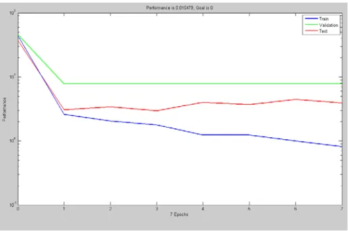
Figure-2 NN plot for Training, Validation and Testing data

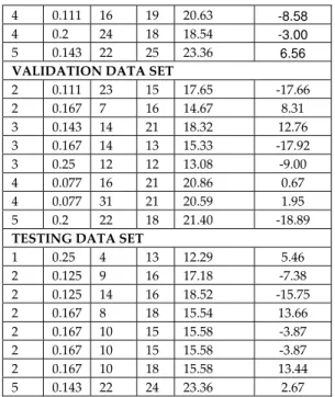
Table II shows the Actual Effort and Feed Forward NN Predicted development time (DT’) and the relative errors.

MC DC LOC DT NN

prediction

(DT ‘)

Error %

TRAINING DATA SET

1 0.25 10 13 12.43 4.38

1 0.333 4 9 9.35 -3.89

2 0.083 10 15 18.84 -25.60

2 0.125 9 15 17.18 -14.53

2 0.2 10 13 14.19 -9.15

2 0.2 10 14 14.19 -1.36

2 0.2 10 15 14.19 5.40

2 0.2 15 13 15.56 -19.69

2 0.25 10 12 12.53 -4.42

3 0.083 17 22 19.89 9.59

3 0.125 11 19 18.18 4.32

3 0.125 15 18 19.08 -6.00

3 0.125 15 19 19.08 -0.42

3 0.143 13 21 18.05 14.05

3 0.143 14 20 18.32 8.40

3 0.143 15 19 18.56 2.32

3 0.143 15 20 18.56 7.20

3 0.167 13 15 17.02 -13.47

3 0.2 18 19 16.75 11.84

3 0.25 9 13 13.32 -2.46

(5)

4 0.111 16 19 20.63 -8.58

4 0.2 24 18 18.54 -3.00

5 0.143 22 25 23.36 6.56

VALIDATION DATA SET

2 0.111 23 15 17.65 ‐17.66

2 0.167 7 16 14.67 8.31

3 0.143 14 21 18.32 12.76

3 0.167 14 13 15.33 ‐17.92

3 0.25 12 12 13.08 ‐9.00

4 0.077 16 21 20.86 0.67

4 0.077 31 21 20.59 1.95

5 0.2 22 18 21.40 ‐18.89

TESTING DATA SET

1 0.25 4 13 12.29 5.46

2 0.125 9 16 17.18 ‐7.38

2 0.125 14 16 18.52 ‐15.75

2 0.167 8 18 15.54 13.66

2 0.167 10 15 15.58 ‐3.87

2 0.167 10 18 15.58 13.44

5 0.143 22 24 23.36 2.67

Table II – Actual Effort(DT) and NN predicted Efforts (DT’)

2.3 Statistical Analysis and Regression Modeling

Before conducting regression analysis we proceed to check if the data was normally distributed. Figure 3 shows a histogram plot of a normally distributed dataset.

(6)

From the dataset, MC, DC and LOC were taken as input and DT as output. A linear regression model was obtained using the commercial package STATISTICA by conducting the stepwise regression modeling. Table III shows the table containing DT predicted through the regression analysis.

Actual (DT)

Predicted by Regression

Analysis

(DT’)

Error %

13.00000 10.85161 16.52607692

9.00000 8.18266 9.081555556

15.00000 18.09036 ‐20.6024

15.00000 17.18999 ‐14.59993333

15.00000 16.73981 ‐11.59873333

16.00000 16.73981 ‐4.6238125

16.00000 15.38925 3.8171875

18.00000 15.38925 14.50416667

15.00000 15.38925 ‐2.595

18.00000 15.38925 14.50416667

13.00000 14.32810 ‐10.21615385

14.00000 14.32810 ‐2.343571429

15.00000 14.32810 4.479333333

13.00000 14.32810 ‐10.21615385

12.00000 12.72030 ‐6.0025

22.00000 19.95905 9.277045455

19.00000 18.60849 2.060578947

18.00000 18.60849 ‐3.3805

19.00000 18.60849 2.060578947

21.00000 18.02969 14.14433333

20.00000 18.02969 9.85155

21.00000 18.02969 14.14433333

19.00000 18.02969 5.106894737

20.00000 18.02969 9.85155

15.00000 17.25794 ‐15.05293333

13.00000 17.25794 ‐32.75338462

19.00000 16.19679 14.75373684

13.00000 14.58899 ‐12.223

12.00000 14.58899 ‐21.57491667

21.00000 22.02067 ‐4.860333333

19.00000 20.92737 ‐10.14405263

18.00000 18.06548 ‐0.363777778

24.00000 21.76707 9.303875

25.00000 21.76707 12.93172

(7)

Table III – Actual Effort (DT) and Regression Analysis Predicted Efforts (DT’)

3. Result and Discussion

A comparison of the 3-3-1 NN output with measured experimental values of effort shows the % error varying from +14.05 to -25.60, +12.76 to -18.89 and +13.66 to -15.75 for the training dataset (25 nos.), validation dataset (8 nos.) and testing dataset (8 nos.), respectively. A much simplified NN architecture was able to effectively and successfully model the non-linear relationship between the 3 variables and a single output parameter. The performance of NN can be further increased by increasing the neurons in the hidden layer and retraining the model with the data. Also the performance will improve with large datasets.

4. Conclusion

In this paper, effectiveness of NN modeling approach of effort estimation for standard dataset was presented. The NN model trained using experimental data was found to have good generalization capabilities and is able to successfully predict the effort closely matching the experimental observations. Since the effect of various cost drivers on effort is often quite complex, ANN can be used as an effective tool to model and predict the development effort. However, the models should also be evaluated by exploring a variety of historical and unseen input data and the model can be adapted and tested to predict the early effort estimation in software development.

5. Running Heads

SDEENNRMA

6. References

[1] C. Lopez-Martin, C.Yanez-Marquez, A.Gutierrez-Tornes, “Predictive accuracy comparison of fuzzy models for software development effort of small programs, The journal of systems and software”, Vol. 81, Issue 6, 2008, pp. 949-960.

[2] C.L. Martin, J.L. Pasquier, M.C. Yanez, T.A. Gutierrez, “Software Development Effort Estimation Using Fuzzy Logic: A Case Study”, IEEE Proceedings of the Sixth Mexican International Conference on Computer Science (ENC’05), 2005, pp. 113-120.

[3] Steve McConnell. Rapid development: taming wild software schedules. Microsoft Press, 1996.

[4] A. Idri, T. M. Khoshgoftaar, A. Abran. “Can neural networks be easily interpreted in software cost estimation?”, IEEE Trans. Software Engineering, Vol. 2, 2002, pp. 1162 – 1167.

[5] A. Idri,, A. Abran,, T.M. Khoshgoftaar. “Estimating software project effort by analogy based on linguistic values” in. Proceedings of the Eighth IEEE Symposium on Software Metrics, 4-7 June 2002, pp. 21 – 30.