Abstract
The purpose of this study is to obtain numerical estimations of seis-mic pressures in offshore areas considering the effect of seabed con-figurations and soil materials. To this end, the Boundary Element Method is used to irradiate waves, so that force densities can be obtained for each boundary element. From this hypothesis, Huygens´ Principle is implemented since the diffracted waves are constructed at the boundary from which they are radiated. Application of bound-ary conditions allows us to determine a system of integral equations of Fredholm type of second kind and zero order. Various models were analyzed, the first one is used to validate the proposed formulation. Other models of ideal seabed configurations are developed to esti-mate the seismic pressure profiles at several locations. The influence of P- and SV-wave incidence was also highlighted. In general terms, it was found that soil materials with high wave propagation velocities generate low pressure fields. The difference between the maximum pressure values obtained for a soil material with shear wave velocity of m/s is approximately 9 times lower than those obtained for a material with 9 m/s, for the P-wave incidence, and 2.5 times for the case of SV-waves. These results are relevant because the seabed material has direct implications on the field pressure ob-tained. A relevant finding is that the highest seismic wave pressure due to an offshore earthquake is almost always located at the sea-floor.
Keywords
Offshore structures, seismic pressures, oil industry, earthquake, elastic waves, Boundary Element Method.
Seismic Pressures in Offshore Areas: Numerical Results
Norberto Flores-Guzmán a
Enrique Olivera-Villaseñor b
Andriy Kryvko c
Alejandro Rodríguez-Castellanos b,c
Francisco Sánchez-Sesma d
a Centro de Investigación en Matemáticas, Jalisco s/n, Mineral de Valenciana, Gua-najuato, GuaGua-najuato, México. Email: [email protected]
b Instituto Mexicano del Petróleo, Mé-xico D F. Eje Central Lázaro Cárdenas 152, Gustavo A. Madero, Distrito Fede-ral, México. Email: [email protected], [email protected]
c Escuela Superior de Ingeniería Me-cánica y Eléctrica, Instituto Politécnico Nacional, ESIME Zacatenco, UPALM, Edif. 5, Av. Instituto Politécnico Nacio-nal S/N, Col. Lindavista, Gustavo A. Madero, Distrito Federal, México. Email: [email protected].
d Instituto de Ingeniería, Universidad Nacional Autónoma de México, Coyoacán, México, Email: [email protected]
http://dx.doi.org/10.1590/1679-78252376
1 INTRODUCTION
Several studies have pointed out that marine seismic activity is considerable. In fact, a large number of seismic movements have epicenters in offshore areas (Mangano et al., 2011). On the other hand, Sasaki et al. (1986) reported that the most intense earthquakes in Japan, which caused great damage, were generated offshore rather than onshore and then they pointed out that installation of seabed sensor is very important to obtain preliminary signs of a destructive earthquake. Additionally, Taka-mura et al. (2003) mentioned that seaquakes are characterized by the propagation of vertical earth-quake motions at the sea bottom as a compression wave and are reported to cause damage to ships and their effect on floating structures is a matter of great concern. With this idea in mind, these authors found an important link between the vibration of the floating structure and the deformation of the seabed when a seaquake takes place.
Marine installations are necessary and seismic effects on them should be taken into account. Marine structures cover a broad range of forms and functions. For instance, submarine pipelines, sea platforms, ships, breakwaters, marine tunnel, among others. In this context, results that contribute to the better understanding of the effects of seismic actions on marine structures are useful to increase the safety level of the offshore industry. Experimental, analytical and numerical methods have been carried out to deal with this issue.
In order to examine the seismic behavior of breakwaters, an analysis of coupled hydrodynamic response characteristics and water pressures on the breakwaters was carried out by a shaking table model test (Uwabe et al. 1983), their results suggest that modeling and material properties are very important factors to simulate the actual field conditions. Moreover, a substructure on-line dynamic testing system used to investigate the interaction between an offshore structure and the foundation soil subjected to seismic loads was developed in (Hyodo et al. 2000). Such study evinced that the residual deformation of the foundation could be attributed to the seismic motion effect. In Jinsi (1985) exhaustive discussions and assessments of field data and their application to submarine pipeline design were carried out. This author investigated on the potential effects of seismic shocks, the strength and lifetime stability of pipelines.
Other field investigations showed that the liquefaction occurred during the 1995 Kobe earthquake may affect the Kobe Harbor´s walls and failures could be expected when the intensity of seismic inertia forces is as strong as the one that was experienced in 1995 (Towhata et al. 1996). On the other hand, experimental studies have been performed as a research project of the Japan Ocean Industries Association to analyze the earthquake induced dynamic water pressure on offshore structures in ice-covered waters (Kobayashi and Kawaguchi 2000). They observed that the earthquake induces dy-namic water pressures, which are greatly increased by the presence of an ice sheet attached around the offshore structure. During the 2003 Tokachi-Oki earthquake, pressure variations were registered by the ocean-bottom observatory located near the epicenter (Le et al., 2009). They reported that acoustic (pressure) waves bouncing up and down between the hard bottom and the sea surface were generated by the seismic seafloor displacement. Their results also evinced that soft sediment layers at the ocean-bottom should be taken into account to estimate accurate pressure values.
spatial spectrum for sea-bottom deformation caused by the earthquake. Kato et al. (2010) reported variations of seismic velocities and converted teleseismic waves that revealed the presence of zones of high-pressure fluids in the subducting Philippine Sea plate in Tokai district, Japan. They pointed out that overpressured fluids appear to be trapped within the oceanic crust by an impermeable cap rock and that such pressures are reduced in zones where permeable soils exist. An autonomous data-acquisition system was installed on the sea floor to record seismic and pressure signals generated by earthquakes and tsunamis (Mangano et al., 2011). In Lipa et al. (2011) pressure-sensor observations of changes in the sea surface elevation and observations of sea level fluctuations at the coast were done in order to obtain warnings of the presence of tsunamis. They also found that the bathymetric effects are very important to determine precise predictions.
Baba, Takahashi and Kaneda (2013) studied the correlation between coastal and offshore tsunami height using an array of ocean-bottom pressure gauges. In this study, ocean-bottom pressure fluctua-tions during tsunamis were obtained, which were also verified by using numerical models. They em-phasized that there is a correlation between the average absolute ocean bottom pressure and tsunami height at the coast. Following this idea, a dense ocean-floor network system for earthquakes and tsunamis started its operation in Nankai Trough, SW Japan in the early of 2010 using various sensors such as broadband seismometer, seismic accelerometer, tsunami meter, etc (Matsumoto et al. 2014; Matsumoto, Kawaguchi and Araki, 2015).
Earthquake induced hydrodynamic pressures acting on the surface of axisymmetric offshore struc-tures were studied by Sun and Nogami (1991). These authors developed a analytical and semi-numerical approach based on the use of a complete and non-singular set of Trefftz functions to de-termine earthquake induced hydrodynamic pressures. In this study, effects of water compressibility, gravity waves on the water surface and the geometrical shape of the structural surface were discussed. A seismic analysis method for floating offshore structures subjected to the hydrodynamic pressures induced from seaquakes was developed by Lee and Kim (2015). Here, the authors applied their method to the seismic analysis of a simplified floating offshore structures, finding that, the dynamic response of the floating offshore structure induced by the vertical seismic motion of the ocean bed can be greatly influenced by the compressibility of the sea water and the energy absorption capability of the seabed.
On the other hand, numerical methods have significant advantages over the other methods like field instrumentations and analytical solutions. For instance, analytical methods frequently treat the problem by simplifications of the reality. Then, an analytic solution is to know absolutely how the model will behave under any circumstances, but it works only for simple models. Field instrumenta-tions are very expensive and the results are limited to the site and condiinstrumenta-tions where they are installed. Numerical methods are mainly used to solve complex problems, physically or geometrically.
plugging resistance was degraded by more than 80%. Additionally, FEM was also used to study the seismic response of underwater storage tanks resting on a horizontal seabed subjected to stochastic earthquake loading (Karadeniz 2007), here the interactive water pressure acting on the tank during the free motion of the tank and earthquake motion was calculated. Moreover, submarine slope stabil-ity was evaluated using a 2D limit equilibrium numerical method. This method allowed to understand that earthquake loading can drastically reduce the shear strength of sediment with increased pore water pressure (Zhang and Luan 2013).
Moreover, the Boundary Element Method (BEM) has been applied to solve problems related to fluid-solid media subjected to seismic excitations. For instance, for the dynamic response of a concrete gravity dam subjected to ground motion and interacting with water, foundation and bottom sediment was studied using the Boundary Elements (Dominguez and Gallego 1996). These authors concluded that the sediment compressibility has a very important effect on the dam response and that the influence of the thickness of the sediment layer is significant. Moreover, Schanz (2001) applied the BEM to study the dynamic responses of fluid-saturated semi-infinite porous continua subjected to transient excitations such as seismic waves. The model allows one to represent continuous media with water, viscoelastic and fluid-filled pore-elastic zones. On the other hand, a special boundary method for earthquake-induced hydrodynamic pressures on rigid axisymmetric offshore structures, including both the water compressibility and seabed flexibility, was presented (Avilés and Li 2001). These authors showed numerical results for different geometries of the structural surfaces. Moreover, the effects of water compressibility and seabed flexibility were examined.
Finally, a boundary integral equation was derived to analyze the seaquake-induced hydrody-namic pressure acting on the floating structure, assuming that the seabed is a semi-infinite homo-geneous elastic solid (Takamura et al. 2003). In their work, they reported that the response char-acteristics of the floating structure largely depend on the vibration properties of the ground surface, and the elastic deformation characteristics of the floating body depend on the rigidity of the floating body and the ground. Moreover, Higo (1997) and Jang and Higo (2004) used boundary integral equations to calculate the hydrodynamic pressure on floating structures caused by seaquakes. In these studies, 2D- and 3D-media were considered and the effect of seaquake forces on the floating structure was emphasized. Qian and Yamanaka (2012) developed the BEM to study the interaction of seismic waves in irregular fluid solid interfaces in multilayered media. To this end, they defined a global matrix with boundary and continuity conditions in such way that they propagate the information of the element displacements and tractions 'downwards' for layers above the source while 'upwards' for layers below the source. The authors pointed out that their method could be applied to offshore wave propagation. Some recent applications of BEM are focused on the seismic amplifications in offshore areas considering the effects of compressional and distortional seismic waves (e.g. Rodríguez-Castellanos et al. 2014). In such work, the seismic amplifications due to simple bathymetric features are highlighted.
and discussed, in frequency and time domain. These pressures are calculated along the water depth at several locations. The following sections describe this formulation.
2 FIELD EQUATIONS IN ELASTODYNAMICS
The basic equations of elastodynamics written according to the classic work of Pao and Mow (1973) are:
Equations of motion:
, , (1)
strain-displacement relations:
, , , (2)
and stress-strain relations:
, (3)
where: x, is the displacement vector at the point x at time t, and are the stress and deformation tensors, respectively, and are the Lame´s constants and ρ is the mass density. The equations are related to a Cartesian coordinate system (i, j=1, 2 ) where indicial notation is used (convention of sum over repeated indices; the commas indicate spacial derivation; and the points means temporary derivation). The Kronecker´s delta is and it is defined as equal to one if i=j and zero if i≠j. In Equation (1) are the body forces.
By combining Equations (1) and (3), one can obtain the Navier equation, having:
, , . (4)
This is the governing equation for an elastic, homogeneous and isotropic solid of volume Ω and surface .
Defining the compressional and shear wave velocity ( and ), respectively, as:
and . (5)
Using Equation (5), it is possible to rewrite Equation (4), as:
, , (6)
These equations are subject to the initial conditions x, and x, in the domain
Ω, with boundary conditions:
x, , x∈
x, , x∈ , (7)
volume. Moreover, it is accepted that the movements and the second order derivatives are continuous (Manolis and Beskos, 1988).
In accordance with the Helmholtz theorem, any displacement field can be expressed as the sum of the gradient of a scalar field and the rotational of a vector field, in such a way that:
, , , (8)
where the alternated tensioner is +1 when the subindexes are in cyclical order (123, 231, 312 ), -1 when they are in acyclic order (321, 213, 132) and 0 when two subindexes are repeated, , .
By replacing the potential representation for in the equation of motion (6), this can be written in terms of the displacement derivatives, neglecting the body forces, as:
,
, (9)
where is the Laplacian operator.
The Lame´s theorem (Aki and Richards, 1980) ensures that each solution of equation (6) is contained in equations (9). In addition, there are only two wave types that propagate in an elastic, infinite and solid medium, one of them given by the vector field φ, which propagates at a velocity and the other given by the field , which propagates at a velocity .
The integral representations, such as those studied in the next section, satisfy equations (9). Once implemented the boundary conditions of the problem, a system of integral equations is formed. This is detailed in the following section.
3 FORMULATION OF THE PROBLEM IN TERMS OF INTEGRAL REPRESENTATIONS
The integral formulation shown in this section gives a numerical solution to obtain pressure variations, with water depth, due to seismic actions. Various seafloor configurations are considered. Schemati-cally, Figure 1 shows an outline of an oil field and illustrates the range of marine structures that are used at different sea depths. The configuration is a ramped one and reaches up to the coastline.
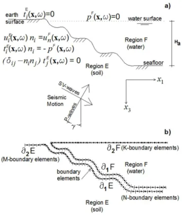
To apply our integral formulation we need to define the boundary conditions and the regions in which the problem is divided (see Figure 2). In Figure 2a, the domain is divided into Region E (soil) and Region F (water). The boundary conditions considered are: traction-free boundary condition at the earth surface, pressure-free boundary conditions at the water surface and continuity of tractions and displacements at the water-soil interface. The incidence of P- and SV-waves is shown schemati-cally in Figure 2a, where Ha is the water depth.
In Figure 2b, the boundary mesh is illustrated. Region E (soil) is delimited by the boundaries
E 1
and E 2
, while Region F is delimited by F 1
and F 2
. Here the variables M, N and K represent the number of boundary elements that are used to discretize the boundaries.
Figure 2: a) Boundary conditions; b) Boundary mesh. The domain is divided into Region E (soil) and F (water) and the variables N, M and K are the number of boundary elements used for the mesh.
Integral representations for the problem studied
x, x, , , x, , , Ω x,
x, x, , , x, , , Ω x, .
(10)
where x, , and x, , are the Green's functions for displacements and tractions, respec-tively, which can be found in Rodriguez-Castellanos et al. (2014); x, and x, are free terms depending on the type of elastic waves impinging on the body (region E), for this study it is the occurrence of P- and SV-waves, x , and , and is the circular frequency. The variables x, represent the receiver and source points, respectively, and are the body forces.
If the body is a fluid, the following functions represent the displacement and pressure fields:
x, x, , , x, , , Ω ,
x, x, , , x, , , Ω , (11)
where x, is the force density for the fluid, is the fluid density, x, , is the Green function for the fluid and is given by x, , ⁄ , is the Hankel function of the second kind and zero order , r is the distance between x and , is the fluid velocity. The superscript F denotes fluid and “i” is the imaginary unit. The subindex “n” in Equations (11) indicates the normal projection of the displacements.
Boundary conditions of the problem
The boundary conditions that have to be imposed to the problem are (see Figure 2a): On the free surface of the water the pressure is zero, i.e.:
x, , ∀x ∈ . (12)
At the free Surface of the earth:
x, , ∀x ∈ . (13)
At the seabed:
Continuity of normal displacements:
x, x, , ∀x ∈ , . (14)
Stresses in the solid are balanced with water pressure:
x, x, , ∀x ∈ , . (15)
Shear stress is zero in solid-water interface:
x, , ∀x ∈ , . (16)
x, , , , (17)
x, , , x, , (18)
x, , , x, , , x, , (19)
x, , , x, , , x, , (20)
x, , , x, . (21)
The variables x, , x, and x, are the incident displacement and traction fields expressed in terms of the normal and tangential ( ) directions to the boundary. Equations (17) - (21) represent the Fredholm´s system of integral equations of 2nd-kind and 0-order to be solved.
3.1 Discretization Scheme of the Boundary Intregral Equations
To numerically solve the system of integral equations (17) – (21), we discretize these properly. In general, the boundaries of each region are discretized into linear segments (N-, M- and K-boundary elements, see Figure 2b) whose size depends on the shortest wavelength (six boundary segments per wavelength). The force densities x, and x, are taken to be constant along each segment and Gaussian integration (or analytical integration, where the Green’s function is singular) is per-formed. The system to be solved is composed of 2(NM)NK equations. Once the system of integral equations is solved, the unknown values of x, and x, are obtained and the dis-placement and pressure fields are computed by means of Equations (11). Region F is between borders
(N-elements) and (K-elements). While, Region E is formed by (N-elements) and (M-elements), see Figure 2b.
Thus, discrete form of Equation (17) can be expressed as:
x , ∑ x , , , for … . (22)
Equation (18) can be written as:
x , ∑ x , , x , , for … , (23)
and Equation (19) as:
x , x , , x , x , ,
x , , for … .
(24)
x , x , , x , x , ,
x , , for … ,
(25)
and Equation (21) as:
x , ∑ x , , x , , for … . (26)
Equations (22) - (26) represent the system of integral equations of Fredholm type of second kind and zero order, which can be solved in frequency domain using Gaussian elimination method and the results in time domain are obtained by means of the Discrete Fourier Transform (DFT) algorithm.
3.2 Application And Remarks of the Boundary Element Method
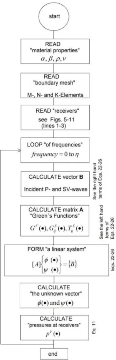
In order to show the application of the method, the following chart (Figure 3) displays the process employed to calculate the seismic pressures at the locations mentioned in Section 5. Basically, the procedure considers the data input, models, locations, Green´s function calculations, forming the system of integral equations, solution and calculus of seismic pressures at the locations. The material properties can be seen in Table 1 and 2. The dimensionless frequency is defined in Section 4.
Many papers have reported advantages and disadvantages about the capability of the application of BEM. One of the most important features of the BEM is that only the boundaries of the region need to be discretized, which leads to a reduce of the amount of elements. Another feature is that it can be used to efficiently solve problems with an infinite or semi-infinite domains and no fictitious boundary conditions need to be established at remote locations. However, some disadvantages of BEM are, for instance, the treatment of the singularities needs special mathematical and numerical techniques to deal with. Moreover, the fundamental solution of the governing equations could be difficult to obtain in some problems.
In this work, the medium, in which the elastic waves propagate, is considered to be an elastic, isotropic and homogenous half space. This medium is divided into regions and is discretized using boundary elements (see Figure 2b). A very fine mesh (considering 6-boundary elements per S- wave-length or higher values) permits having detailed geometries to be studied. In respect to the model size, only a finite part of the water and interfaces need to be modeled. Such truncation brings artificial perturbations produced by diffractions at the edges of the numerical model. Nevertheless, these per-turbations are characterized by small amplitudes and their reflections inside the model are negligible. The simplest solution is to choose a surface length large enough that the fictitious perturbations fall outside of the observational space-time window.
Figure 3. Flow chart. Procedure to illustrate the application of the Boundary Element Method to calculate seismic pressures.
4 VERIFICATION OF THE METHOD
We define , as Wong and Kawase did, where "a" is the radius of the semi-circular canyon, ω is the circular frequency and is the shear wave velocity of the elastic solid. If we consider and . (Poisson ratio) and plot the calculated seismic amplifications on the canyon semi-circular surface between (see reference system in Figure 2a), our results are in good agreement with those obtained by Wong and Kawase.
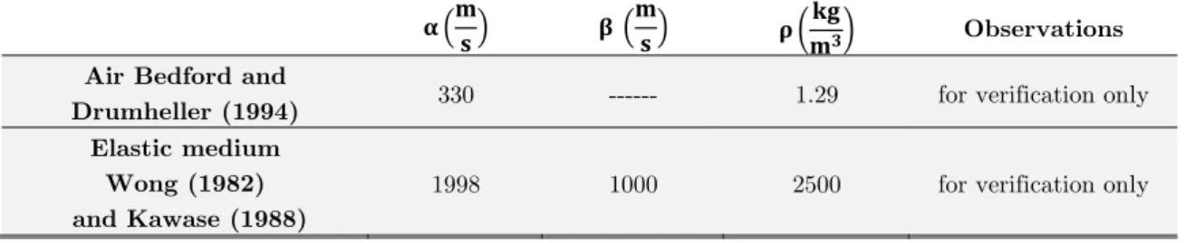
To reproduce those results, the incidence of P and SV-waves with an angle of ° is employed. The elastic properties ( , and ) used in this verification process are shown in Table 1.
Observations Air Bedford and
Drumheller (1994) 330 --- 1.29 for verification only
Elastic medium Wong (1982) and Kawase (1988)
1998 1000 2500 for verification only
Table 1: Elastic properties for elastic and acoustic media used for verification. These parameters were used to reproduce the Wong´s and Kawase´s results.
In Figure 4, our results are plotted with solid lines (horizontal component) and with dashed ones (vertical component). Circles correspond to Wong´s results, and squares to Kawase´s results. It is noteworthy that the largest seismic amplifications, for the vertical component, are present for the P-waves incidence, showing values close to 2.8 at at and . The lower amplifications are present at , . The amplifications associated to the horizontal component are always less than 1 within the range of . In the case of SV waves, the largest seismic amplifications are observed for the horizontal component, reaching values of 2.9 at . and . . The vertical component presents values greater than 1 but less than 2 for the range of and . In general, it is pointed out that a topography causes seismic amplifications near 3.
Figure 4: Seismic amplification for a semicircular topography. Circles represent results obtained by Wong (1982) and squares by Kawase (1988). Results from the current formulation are plotted with
5 SEISMIC PRESSURES FOR SEVERAL NUMERICAL MODELS
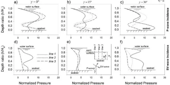
Using the same elastic properties as in the previous case, the seismic pressure profiles for three lines (1 to 3) for a simple seafloor configuration (see Figures 5e and 6e) have been calculated. Hereafter, the material properties (fluid and solid) are divided by the material properties of the solid in order to present dimensionless pressures in the plotted results. Water´s properties are: weight (1020 kg/m3) and wave velocity (1500 m/s2). Figures 5 and 6 show the pressure profiles for P- and SV-wave incidences with angles of °, 15° and 30°. Line 1 is located near the vertical cliff, lines 2 and 3 are located at a distance of Ha and 2Ha to the vertical cliff, respectively (see Figures 5e, 6e), where Ha is the water depth.
Figure 5 shows the dependence of pressures with respect to frequency, in this case . There are complex pressure patterns, which depend mainly on the line location and the incident wave type. For example, according to the pressures caused by the P wave incidence, the maximum pressure reached is less than 15 to a depth of . (see Figure 5c, Line 1). In the case of °and 15°, Line 3 (dashed) reaches pressure values close to 14 near to a depth of . (see Figures 5a, b).
Figure 5: Seismic pressure profile for a simple seabed configuration for . The incidence of P- and SV-waves for °, ° and ° is considered.
Figure 6: Seismic pressure profile for a simple seabed configuration for . The incidence of P- and SV-waves for °, ° and ° is considered.
Figures 7 and 8 show the influence of a ramped sea floor configuration on the pressure field. The elastic properties are similar to those of the previous figures. We studied the P- and SV-waves inci-dence with an inciinci-dence angle of °. For all these figures the pressures due to the incidence of P-waves are plotted with a solid line and the corresponding to the SV P-waves with a dashed one. The ramp slopes are represented by , which takes the values of °, 45° and 60° (up, middle, and down figures). Again, the pressures are obtained for Lines 1, 2 and 3 (see details at the bottom of each figure). In these figures, one can notice a clear dependence of pressures with respect to the frequency ( and 4).
For (Figure 7), pressures can reach values less than 20 and it can be seen that the P-wave incidence causes greater pressures than SV-waves. Moreover, Line 3, in general, has the highest pres-sures, reaching a value of 20 on the ocean floor for an angle ° (Figure 7i). For (Figure 8), more oscillations are present and normalized pressure values greater than those for are observed, this is due to the increase in frequency. In this case, the maximum normalized pressure values are 50 (see Figure 8f) and 40 (see Figures 8c and 8i) located on the seafloor. Once more, the P-wave incidence generates the greatest pressure field.
Figure 7: Seismic pressure profile for a ramped seabed configuration for . The normal incidence of P- and SV-waves is considered. Higher seismic pressures are observed at Line 3 in all cases.
Influence of the sea floor´s soil properties on the pressure field
Figure 8: Seismic pressure profile for a simple seabed configuration for . The normal incidence of P- and SV-waves is considered. Higher seismic pressures are observed at Line 3 in all cases.
Material
SV-wave velocity ( ) (m/sec)
Density ( ) (kg/m3)
Poisson´s ratio
( )
Reference
1 3000 2100 0.25
Huerta-Lopez et al. (2003)
2 400 1700 0.35
3 190 1400 0.40
4 90 1300 0.45
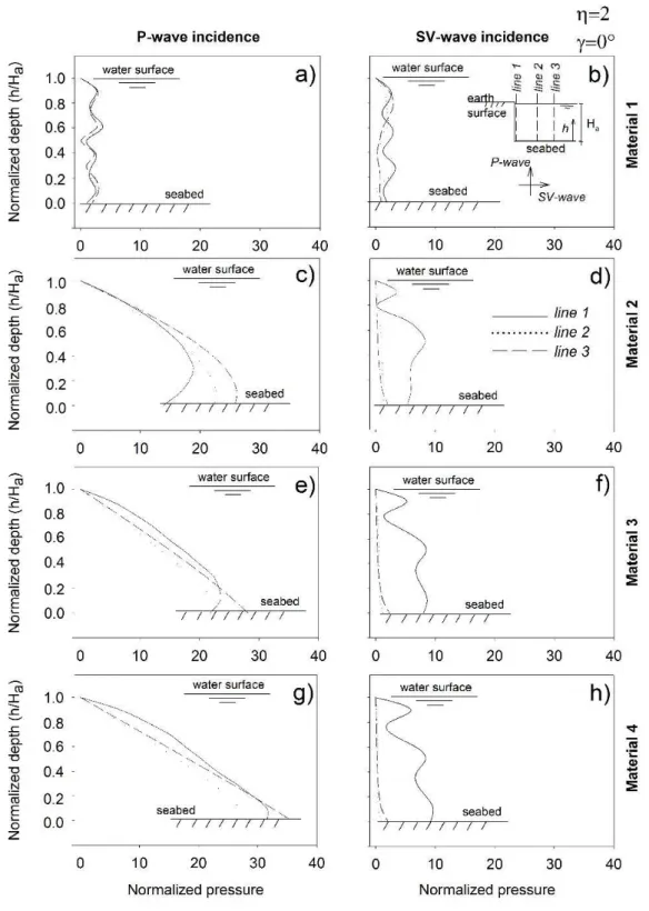
Figure 9 shows the pressure field obtained for the configuration shown in Figure 9b. In this example, normal P- and SV- wave incidence ( °) is considered. Four types of materials for the seabed were modeled, which are shown in Table 2. The frequency analyzed is . The pressures for each case are obtained for lines 1 to 3 (location of such lines is the same as in Figures 5 and 6, line 1 is located near the vertical cliff, lines 2 and 3 are located at a distance of Ha and 2Ha to the
vertical cliff, respectively). The highest wave velocity ( m/s) of Material 1 can be associ-ated with a high rigidity of the medium. This could be a relevant characteristic that distinguishes Material 1 from the other materials in Table 2. As shown in Figure 9a and 9b the values of the pressure field are lower for this material and, essentially the lines 1 to 3 have the same magnitudes and patterns. For the other three materials it may be inferred from the results, that the lower wave velocity β (i.e. Material 4) generates the greatest pressure field. This is observed for both P- and SV-wave incidences. For instance, Material 4 (see Figure 9g) reaches values of 37 on the seabed, for the incidence of P-waves. This value is lower for Material 3 and even less than for Material 2. In fact, for the SV-wave incidence a similar behavior is observed. The material with lower wave velocity (i.e. 9 m/s) generates greater pressures. The maximum pressures are also found in the proximity of the seafloor and correspond to the material 4. It should be noted that the pressures obtained in lines 2 and 3 are almost negligible for the SV-wave incidence and for any material of the seafloor. In all cases, this figure shows null pressures at the water surface, as expected. There-fore, it could be concluded that a material with higher wave propagation velocity generates a lower values of pressure field, according to the results shown in this figure. The difference between the maximum pressure values obtained for Material 1 is approximately 9 times lower than those ob-tained for Material 4, for the P-wave incidence, and 2.5 times for the case of SV-waves. This result is relevant because the material type that of the seabed has direct implications on the pressure field obtained.
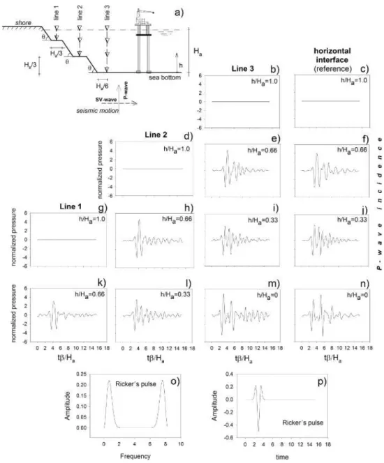
Finally, Figures 10 and 11 present synthetic seismograms of calculated pressures at the receivers shown in Figures 10a and 11a. The material properties considered are the same as those for Figures 4 to 7. To this end, we have used a Ricker pulse with the features, in frequency and time, as illustrated in Figures 10o, 10p, 11o and 11p. The Ricker pulse has a characteristic period of 0.77 sec. For all the cases with h/Ha=1.0, null pressures are obtained (see Figures 10b, 10d and 10g).
This result is consistent with the expected pressures on the water surface. In the right hand column of Figure 10 and 11, the results of pressures generated by the normal incidence of P- and SV-waves on a horizontal interface are displayed, respectively. These last curves are present as a reference.
Figure 10: Synthetic seismograms of pressures for a ramped seabed configuration under the incidence of P-waves. The receivers, where the pressure fields are calculated, are indicated with triangles in the subplot a).
Figure 11: Synthetic seismograms of pressures for a ramped seabed configuration under the incidence of SV-waves. The receivers, where the pressure fields are calculated, are indicated with triangles in the subplot a).
6 CONCLUSIONS
It has been found that the compressional waves (P-waves) can produce greater seismic pressures than the distortional waves (SV-waves). Moreover, P-wave incidences generate greater pressures in remote locations from vertical cliffs. On the other hand, the maximum pressures caused by SV-waves are present in locations close to vertical cliff. The difference between the maximum pressure values obtained for a material with shear wave velocity of m/s is approximately 9 times lower than those obtained for a material with a of 9 m/s, for the P wave incidence, and 2.5 times for the case of SV-waves. This result is relevant because the seabed material type has direct implications on the pressure field obtained. Results in time domain suggest that the calculated pressures are similar to those obtained for a horizontal configuration of the seafloor, for the case of P-waves and for the analyzed configurations. That is to say that the seafloor configuration does not cause great diffractions of P-waves. While, the obtained pressures, when a normal SV-wave excites a ramped configuration, are consequence of the diffractions of SV-waves by the seabed configuration, only. Another relevant finding is that the highest seismic pressure due to an offshore earthquake is almost always located at the seafloor.
The results obtained in this article could be used for the analysis and design of offshore structures. Applications such as the study of pressures on submarine pipelines, marine foundations, pressures on tension-leg platforms and on ships mooring systems could have practical interest.
References
Aki, K., Richards, P.G., (1980). Quantitative Seismology, W.H. Freeman, San Francisco.
Avilés, J., Li, X., (2001). Hydrodynamic pressures on axisymmetric offshore structures considering seabed flexibility. Computers and Structures 79: 2595-2606.
Baba, T., Takahashi, N., Kaneda, Y., (2013). A numerical study for relationship between coastal tsunami and bottom pressure fluctuation in the ocean generated from near-field earthquake, 2013 IEEE International Underwater Technol-ogy Symposium, UT 2013, 2013, 2013 IEEE International Underwater TechnolTechnol-ogy Symposium, UT 2013.
Banerjee, P.K., Butterfield, R., (1981). Boundary Element Methods in engineering science. Mc.Graw Hill. London. Bedford, A., Drumheller, D.S., (1994). Introduction to elastic wave propagation: John Wiley & Sons, Chichester. Choi, Y., Nam, M.S., O'Neill, M.W., (2000). Response of open-ended piles in sand to simulated earthquake and sea-quake. International Journal of Offshore and Polar Engineering 10:229-235.
Dominguez, J., Gallego, R., (1996). Earthquake response of gravity dams including effects of porous sediments. Pro-ceedings of Engineering Mechanics, v 2, p 649-652, 1996; Conference: ProPro-ceedings of the 1996 11th Conference on Engineering Mechanics. Part 1 (of 2), May 19, 1996 - May 22, 1996; Sponsor: ASCE; Publisher: ASCE.
Higo, Y., (1997). Theoretical study on the effect of seaquakes on a two-dimensional floating body. Proceedings of the International Offshore and Polar Engineering Conference 4:480-484.
Huerta-Lopez, C., Pulliam, J., Nakamura, Y., (2003). In Situ Evaluation of Shear-Wave Velocities in Seafloor Sedi-ments with a Broadband Ocean-Bottom Seismograph. Bull. Seism. Soc. Am. 93:139-151.
Hyodo, M., Yamamoto, S., Fukuda, K., Kamesaki, K., Yamauchi, Y., (2000). Behaviour of sand seabed underneath a gravity offshore structure subjected to ice load and seismic force. Proceedings of the International Offshore and Polar Engineering Conference, v 1, p 555-561, 2000; Conference: Proceeedings of the 10th International Offshore and Polar Engineering Conference, May 28, 2000 - June 2, 2000; Sponsor: ISOPE; Publisher: ISOPE.
Jinsi, B.K., (1985). Offshore construction report/soil, seismic studies essential for (submarine pipe) lines in earthquake areas. Oil and Gas 83:72-73.
Karadeniz, H., (2007). Stochastic earthquake-analysis of underwater storage tanks. 26th ASME Offshore Mechanics and Arctic Engineering International Conference [OMAE2007] (San Diego, CA, 6/10-15/2007) Proceed, 2007; ISBN-10: 0791837998.
Kato, A., Iidaka, T., Ikuta, R., Yoshida, Y., Katsumata, K., Iwasaki, T., Sakai, S.I., Thurber, C., Tsumura, N., Yamaoka, K., Watanabe, T., Kunitomo, T., Yamazaki, F., Okubo, M., Suzuki, S., Hirata, N., (2010). Variations of fluid pressure within the subducting oceanic crust and slow earthquakes, Geophysical Research Letters 37, N 14. Kawase, H., (1988). Time-domain response of a semicircular canyon for incident SV, P, and Rayleigh waves calculated by the discrete wave number boundary element method. Bull. Seism. Soc. Am. 78:1415-1437.
Kobayashi, H., Kawaguchi, H., (2000). Evaluation of seismic load on offshore structure in ice-covered waters. Proceed-ings of the International Offshore and Polar Engineering Conference 1:674-678.
Lee, J.H., Kim, J.K., (2015). Dynamic response analysis of a floating offshore structure subjected to the hydrodynamic pressures induced from seaquakes, Ocean Engineering 101:25-39.
Li, W., Yeh, H., Hirata, K., Baba, T., (2009). Ocean-bottom pressure variations during the 2003 Tokachi-Oki earth-quake, Selected Papers of the Symposium Held in Honor of Philip L-F Liu's 60th Birthday - Nonlinear Wave Dynamics, p 109-126, 2009, Selected Papers of the Symposium Held in Honor of Philip L-F Liu's 60th Birthday -Nonlinear Wave Dynamics.
Lipa, B., Barrick, D., Saitoh, S.I., Ishikawa, Y., Awaji, T., Largier, J., Garfield, N., (2011). Japan tsunami current flows observed by HF radars on two continents. Remote Sensing 3:1663-1679.
Mangano, G., D'Alessandro, A., D'Anna, G., (2011). Long term underwater monitoring of seismic areas: Design of an ocean bottom seismometer with hydrophone and its performance evaluation. OCEANS 2011 IEEE – Spain.
Manolis, G.D., Beskos, D.E., (1988). Boundary Element Methods in Elastodynamics, Unwin Hyman, Londres. Matsumoto, H., Araki, E., Kawaguchi, K., Nishida, S., Kaneda, Y., (2014). Long-term features of quartz pressure gauges inferred from experimental and in-situ observations. OCEANS 2014 - TAIPEI, 4 pp., 2014; ISBN-13: 978-1-4799-3646-5; DOI: 10.1109/OCEANS-TAIPEI.2014.6964447; Conference: OCEANS 2014 - TAIPEI, 7-10 April 2014, Taipei, Taiwan; Publisher: IEEE, Piscataway, NJ, USA.
Matsumoto, H., Kawaguchi, K., Araki, E., (2015). Initial characteristics of pressure sensors, 2015 IEEE Underwater Technology, UT 2015, May 14, 2015.
Pao, Y.H., Mow, C.C., (1973). Diffractions of Elastic Waves and Dynamic Stress Concentrations, New York, Crane Russak.
Qian, Z.H., Yamanaka, H., (2012). An efficient approach for simulating seismoacoustic scattering due to an irregular fluid solid interface in multilayered media, Geophysical Journal International 189:524-540.
Rodríguez-Castellanos A., Martínez-Calzada V., Rodríguez-Sánchez, J.E., Orozco-del-Castillo, M., Carbajal-Romero, M., (2014). Induced water pressure profiles due to seismic motions. Applied Ocean Research 47:9-16.
Saito, T., Matsuzawa, T., Obara, K., Baba, T., (2010). Dispersive tsunami of the 2010 Chile earthquake recorded by the high-sampling-rate ocean-bottom pressure gauges, Geophysical Research Letters 37, N 23.
Sasaki, K., Kawasoe, T., Fujisawa, T., (1986). Seabed sensors and their applications to earthquake prediction. Journal of the Institute of Electronics and Communication Engineers of Japan 69:842-845.
Schanz, M., (2001). Application of 3D time domain boundary element formulation to wave propagation in poroelastic solids: Engineering Analysis with Boundary Elements 25:363-376.
Takamura, H., Masuda, K., Maeda, H., Bessho, M., (2003). A study on the estimation of the seaquake response of a floating structure considering the characteristics of seismic wave propagation in the ground and the water. Journal of Marine Science and Technology 7:164-174.
Towhata, I., Ghalandarzadeh, A., Sundarraj, K.P., Vargas-Monge, W., (1996). Dynamic failures of subsoils observed in waterfront areas. Soils and Foundations, in Special, 1996:149-160, Jan 1996; ISSN: 00380806; Publisher: Japanese Soc of Soil Mechanics & Foundation Engineering.
Uwabe, T., Noda, S., Tsuchida, H., (1983). Coupled Hydrodynamic Response Characteristics And Water Pressures Of Large Composite Breakwaters. National Bureau of Standards, Special Publication, p 193-217, 1983; ISSN: 00831883; Conference: Wind and Seismic Effects, Proceedings of the 14th Joint Panel Conference of the US-Japan Cooperative Program in Natural Resources. Sponsor: NSF, Washington, DC, USA; Publisher: NBS.
Wong, H.L., (1982). Effect of surface topography on the diffraction of P, SV; and Rayleigh waves. Bull. Seism. Soc. Am. 72:1167-1183.