and Physics
Retrieving global aerosol sources from satellites using inverse
modeling
O. Dubovik1,2, T. Lapyonok3,4, Y. J. Kaufman5, M. Chin5, P. Ginoux6, R. A. Kahn5,7, and A. Sinyuk3,4 1Laboratoire de Optique Atmosph´erique, Universit´e de Lille 1/CNRS, Villeneuve d ’Ascq, France
2Substantial part of this study was done while worked at: Laboratory for Terrestrial Physics, NASA Goddard Space Flight
Center, Greenbelt, MD, USA
3Laboratory for Terrestrial Physics, NASA Goddard Space Flight Center, Greenbelt, MD, USA 4Science Systems and Applications, Inc., Lanham, MD, USA
5Laboratory for Atmospheres, NASA Goddard Space Flight Center, Greenbelt, MD, USA 6Geophysical Fluid Dynamics Laboratory, NOAA, Princeton, NJ, USA
7Geophysical Jet Propulsion Laboratory, Pasadena, CA, USA
Received: 22 November 2006 – Published in Atmos. Chem. Phys. Discuss.: 12 March 2007 Revised: 4 October 2007 – Accepted: 4 December 2007 – Published: 18 January 2008
Abstract. Understanding aerosol effects on global cli-mate requires knowing the global distribution of tropospheric aerosols. By accounting for aerosol sources, transports, and removal processes, chemical transport models simulate the global aerosol distribution using archived meteorological fields. We develop an algorithm for retrieving global aerosol sources from satellite observations of aerosol distribution by inverting the GOCART aerosol transport model.
The inversion is based on a generalized, multi-term least-squares-type fitting, allowing flexible selection and refine-ment of a priori algorithm constraints. For example, limita-tions can be placed on retrieved quantity partial derivatives, to constrain global aerosol emission space and time variabil-ity in the results. Similarities and differences between com-monly used inverse modeling and remote sensing techniques are analyzed. To retain the high space and time resolution of long-period, global observational records, the algorithm is expressed using adjoint operators.
Successful global aerosol emission retrievals at 2◦×2.5◦ resolution were obtained by inverting GOCART aerosol transport model output, assuming constant emissions over the diurnal cycle, and neglecting aerosol compositional dif-ferences. In addition, fine and coarse mode aerosol emis-sion sources were inverted separately from MODIS fine and coarse mode aerosol optical thickness data, respectively. These assumptions are justified, based on observational cov-erage and accuracy limitations, producing valuable aerosol source locations and emission strengths. From two weeks of daily MODIS observations during August 2000, the global placement of fine mode aerosol sources agreed with available Correspondence to:O. Dubovik
independent knowledge, even though the inverse method did not use any a priori information about aerosol sources, and was initialized with a “zero aerosol emission” assumption. Retrieving coarse mode aerosol emissions was less success-ful, mainly because MODIS aerosol data over highly reflect-ing desert dust sources is lackreflect-ing.
The broader implications of applying our approach are also discussed.
1 Introduction
Knowledge of the global distribution of tropospheric aerosols is important for studying the effects of aerosols on global cli-mate. Satellite remote sensing is the most promising way to collect information about global aerosol distributions (King et al., 1999; Kaufman et al., 2002). However, in spite of recent advances in space technology, the satellite data do not yet provide the required accuracy nor the level of detail needed to assess aerosol property time and space variabil-ity. Tropospheric aerosols may display strong local varia-tions, and any single satellite instrument needs at least sev-eral days of observations to obtain sufficient cloud-free im-ages for global coverage. Also, most satellite aerosol data records are limited to daytime, clear-sky conditions. Com-prehensive, global atmospheric aerosol simulations having adequate time and space resolution can be obtained using global models that rely on estimated emissions and account for aerosol transport and removal processes.
At present, there are a number of well-established Global Circulation Models (GCMs) that generate their own meteo-rology (e.g. models by Roechner et al., 1996; Tegen et al.,
1997, 2000; Koch et al., 1999; Koch, 2001; Ghan et al., 2001a, b; Reddy and Boucher, 2004) and Chemical Trans-port Models (CTMs) that incorporate meteorological data from external sources into the model physics (e.g. models by Balkanski et al., 1993; Chin et al., 2000, 2002; Ginoux et al., 2001; Takamura et al., 2000, 2002). However, the ac-curacy of global aerosol models is limited by uncertainties in aerosol emission source characteristics, knowledge of at-mospheric processes, and the meteorological field data used. As a result, even the most recent models are mainly expected to capture only the principal global features of aerosol trans-port; among different models, quantitative estimates of av-erage regional aerosol properties often disagree by amounts exceeding the uncertainty of remote sensing aerosol obser-vations (e.g. Kinne et al., 2003, 2006; Sato et al., 2003). Therefore, there are diverse, continuing efforts to harmonize and improve global aerosol modeling by refining the meteo-rology, atmospheric process representations, emissions, and other modeling components used.
The availability of aerosol remote sensing products, es-pecially global aerosol fields provided by satellite observa-tions, is of critical importance for verifying and constrain-ing aerosol models. For example, the direct comparisons of model outputs with observed aerosol properties are used for evaluating model accuracy and for identifying possible mod-eling problems (e.g. Takamura et al., 2000; Chin et al., 2002, 2003, 2004; Kinne et al., 2003, 2006). The observations can also be used to optimize the agreement between tracer transport model predictions and observation. For example, model predictions can be adjusted and enhanced by assimi-lating observations into the model. Collins et al. (2000, 2001) improved regional aerosol model predictions by assimilat-ing the available satellite retrievals of aerosol optical thick-ness. Weaver et al. (2006) suggested a procedure for assimi-lating satellite-level radiances into a radiative transfer model driven by GOCART global transport model aerosol field pre-dictions. Another way of improving global aerosol modeling is retrieving (or adjusting) aerosol emissions from available observations by inverting a global model. This approach is particularly promising because aerosol emission uncertainty is widely recognized as a major factor limiting global aerosol model accuracy. It has been shown that inversion techniques are rather effective at improving the accuracy of trace gas chemical models (e.g. Kaminski et al., 1999b; Khattatov et al., 2000; Kasibhatla et al., 2000; Elbern et al., 1997; Para et al., 2003).
However, implementing the same techniques for inverting aerosol models appears to be more challenging. Indeed, a de-scription of the aerosol field generally requires a larger num-ber of parameters compared to a description of atmospheric gases, partly because of relatively high aerosol temporal and spatial variability (see discussion in Sect. 2.5). In addition, direct implementation of basic inversion methods (that use the Jacobi matrices of first derivatives) is computationally de-manding and, therefore, hardly applicable in aerosol global
modeling. In these regards, designing an inversion in a var-tiational formalism framework, using adjoint operators, is rather promising. The adjoint operators (Marchuk, 1977, 1986; Cacuci, 1981; Tarantolla, 1987) allow direct calcu-lation of the gradients of the quadratic form in respect to model input parameters, without explicit use of Jacobi ma-trices. Such calculations have computational requirements similar to those of forward modeling. Correspondingly, us-ing adjoint operators allows efficient implementation of the model inversion by minimizing quadratic form (quantifying mismatch between observations and modeling results) with the gradient methods, provided the methods converge rapidly enough.
Adjoint techniques are widely used in meteorology and oceanography for variational data assimilation (Le Dimet and Talagrand, 1986; Talagrand and Courtier, 1987; Courtier and Talagrand, 1987; Navon, 1997, etc.), and have been success-fully applied to inverse modeling analyses involving atmo-spheric gases (Kaminski et al., 1999a; Elbern et al., 2000; Menut et al., 2000; Vukicevic and Hess, 2000; Vautard et al., 2000; Elbern and Schmidt, 2001; Schmidt and Martin, 2003; Menut, 2003; Elbern et al., 2007). Hakami et al. (2005) used an adjoint approach to retrieve regional sources of black car-bon from aircraft, shipboard, and surface black carcar-bon mea-surements collected during the ACE-Asia field campaign.
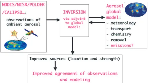
Our paper explores the possibility of deriving the global distribution and strength of aerosol emission sources from satellite observations, using the adjoint operator formula-tion to invert an aerosol transport model. Figure 1 illus-trates the general retrieval concept. In addition, we ana-lyze possible parallels and analogies between inverse mod-eling and retrieval approaches widely used in atmospheric remote sensing. Such analyses may be useful sources of ef-ficient methods developed in remote sensing, that could be adapted to inverse modeling. For example, numerous remote sensing applications use the Phillips-Tikhonov-Twomey in-version technique developed in the early sixties by Phillips (1962), Tikhonov (1963) and Twomey (1963). The technique suggests constraining ill-posed problems using a priori limi-tations on the derivatives of the retrieved function. Here, we discuss the possibility of constraining temporal and/or spatial aerosol variability by applying a priori limitations on aerosol mass derivatives with respect to time and space coordinates. Also, we formulate the inversion problem using a multi-term least squares approach, convenient for including multiple a priori constraints in the retrieval (Dubovik, 2004).
We applied our approach to retrieving global aerosol sources by inverting the Goddard Chemistry Aerosol Radi-ation and Transport (GOCART) model. Algorithm perfor-mance is illustrated by numerical tests, as well as by deriv-ing global aerosol emissions, applyderiv-ing the algorithm to actual MODIS aerosol observations. The algorithms potential and limitations are also discussed more generally.
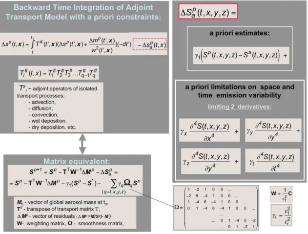
Fig. 1.Flowchart of the retrieval scheme concept.
2 The methodology of inverse modeling
The spatial and temporal behavior of atmospheric stituents is simulated in chemistry models by solving the con-tinuity equation (Brasseur et al., 1999; Jacob, 1999):
∂m
∂t = −v∇m+
∂m
∂t
diff
+
∂m
∂t
conv
+S−R, (1)
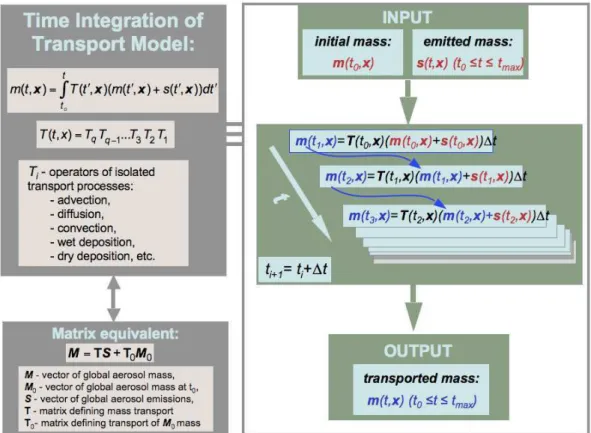
where v is the transport velocity vector, m is mass and suffixes “diff” and “conv” denote turbulent diffusivity and convection, respectively. S and R denote source and loss terms, respectively. The characteristics m, v, S andR in Eq. (1) are explicit functions of timetand spatial coordinates x=(x, y, z). The continuity equation does not yield a general analytical solution and is usually solved numerically using discrete analogues. Each component process in the numeri-cal equivalent of Eq. (1) is isolated and treated sequentially at each time step1t (e.g. Jacob, 1999):
m (t+1t,x)=T (t,x) (m (t,x)+s (t,x)) 1t, (2) wheres(t,x)– mass emission,T (t,x)is transport operator, that can be approximated as:
T (t,x)=TqTq−1...T3T2T1 , (3)
andTi (i=1,. . . ,q)are operators for isolated transport pro-cesses such as advection, diffusion, convection and wet scav-enging. Thus, the calculation of mass at any given time can be reduced to the numerical integration of known transport and source functions:
m (t,x)= t Z
t0
T t′,x m t′,x+s t′,xdt′. (4)
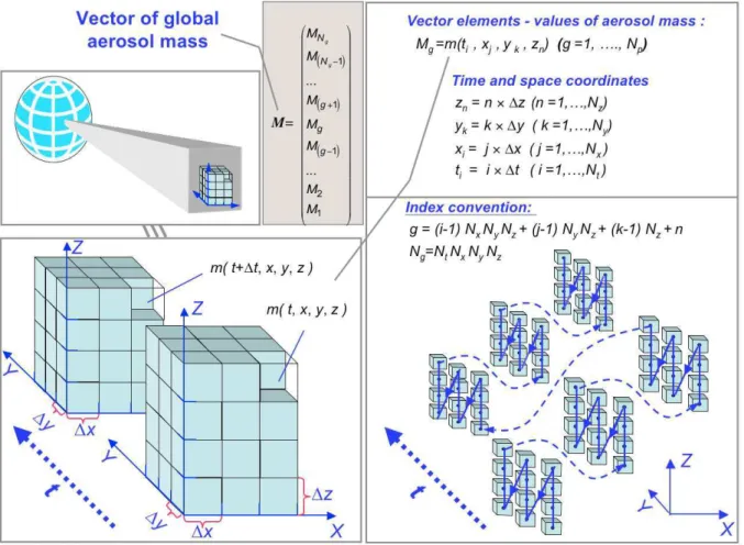
If the transport operator T (t,x) is linear, Eq. (4) can be equivalently written in terms of the matrix equation. For ex-ample, Fig. 2 illustrates one of many possible approaches to representing the global mass distribution by a vectorM. Us-ing the same approach for representUs-ing the global emission distribution by a vectorS, the matrix equivalent of Eq. (4) can be written as (see explicit derivation in Appendix B):
M =TS+T0M0, (5)
whereM0is a vector of mass values at all locations at timet0; MandSare the corresponding vectors of mass and emission values at all locations and considered timest0,t1,. . . ,tn−1,tn (i.e. these vectors represent the 4-dimensional (4D) aerosol mass and emission variability); Tis the coefficient matrix defining the mass transport to each locationx and time step tk from all locationsx and previous time stepsti<n. T0 is
the coefficient matrix defining the transport of mass to each locationxand time steptk from mass present at all locations xand at time stept0. Figure 3 illustrates the relation between
integral Eq. (4) and the representation of aerosol transport modeling in vector-matrix form by Eq. (5). Thus, the source vector can be retrieved by solving the matrix equation if the mass measurementsMmeas=M+1
Mare available.
Using Eq. (5), the inversion of aerosol transport can be implemented numerically as the solution of a system of algebraic equations. However, vectors M, S and matrix
T can have extremely large dimensions (see discussion in Sect. 2.5), and direct implementation of some matrix op-erations can be difficult. Therefore, inverting the transport equation is commonly formulated in a calculus of varia-tions framework, a field of mathematics that deals with func-tions of funcfunc-tions. In this formalism, emission estimation is achived using 4D-variational (4D-var) data assimilation tech-niques (e.g. Le Dimet and Talagrand, 1986; Talagrand and Courtier, 1987; Courtier and Talagrand, 1987; Elbern et al.,
75
Fig. 2.Illustration representing the aerosol global mass distribution in vector form.2000; Vukicevic and Hess, 2000; Elbern and Schmidt, 2001; Schmidt and Martin, 2003; Menut, 2003; etc.). Neverthe-less, here we invert the transport equation using the matrix formulation given by Eq. (5), to retain full analogy with re-mote sensing inversion approaches. We hope this analogy will highlight the parallels between these two research areas, and will make it easier to identify positive developments in remote sensing that can be applied to inverse modeling algo-rithms. Thus, below we discuss the inversion of the transport equation as a formal linear system inversion problem, shown in Eq. (5).
2.1 Statistical optimization of the linear inversion
If the statistical behavior of the errors1M is known, one can use this knowledge to optimize the solution of Eq. (5). In that way, the solutionSˆ should not only closely repro-duce observationsMmeas, but in addition, the remaining de-viations1ˆM=Mmeas−M(Sˆ)should have a distribution close to the expected error properties described by the Probabil-ity DensProbabil-ity Distribution (PDF) of errors P(1M). According to the well-known Method of Maximum Likelihood (MML),
the optimum solution Sˆ corresponds to a maximum of the PDF as follows (e.g. Edie et al., 1971):
P (1M)=P (Mmeas−M(S))=P (M(S)|Mmeas)=max. (6) Where the PDF P(M(S)|Mmeas), written as a function of re-trieval parametersSfor a given set of available observations Mmeas, is known as a Likelihood Function. The MML is a
fundamental principle of statistical estimation that provides a statistically optimum solution in many senses. For example, the asymptotic error distribution (infinite number of1M re-alizations) of MML estimates has the smallest possible vari-ance. Most statistical properties of the MML solution remain optimal for a limited number of observations (e.g. see Edie et al., 1971). The normal (or Gaussian) distribution is widely considered as the best model for describing actual error dis-tribution (Tarantola, 1987; Edie et al., 1971; etc.):
P M(S)|Mmeas= (2π )mdet(CM) −1/2 exp
−1
2 M(S)−M
measT
C−M1 M(S)−Mmeas
, (7) where (. . . )Tdenotes matrix transposition,CM is the covari-ance matrix of1M, det(C) denotes the determinant ofCM,
76
Fig. 3.Illustration of the relation between sequential time integration of aerosol transport and the representation of aerosol transport modeling in vector-matrix form.
and m is the dimension of the vectors M(S) and Mmeas.
The maximum of the PDF exponential term in Eq. (7) cor-responds to the minimum of the quadratic form in the expo-nent. Therefore, the MML solution is a vectorSˆ correspond-ing to the minimum of the followcorrespond-ing quadratic form:
9 (S)=1
2 M(S)−M
measT
C−M1 M(S)−Mmeas
=min. (8) Thus, with the assumption of normal noise, the MML prin-ciple requires searching for a minimum in the product of the squared terms of(Mmeas −M(S))in Eq. (7). This is the basis for the widely known Least Square Method (LSM).
For linearM(S)(as in Eq. 5), the LSM solution can be written as (e.g. Rao 1965):
ˆ
S=TTC−m1T−1TTC−m1M∗. (9) Here,M∗is the vector of mass measurements corrected for the backdround aerosolM0present in the atmosphere at t0
(i.e. prior observations):M∗=Mmeas–TM 0.
2.2 Inversion constrained by a priori estimates of un-knowns
If the problem is ill-posed and Eq. (5) does not have a unique solution, then some a priori constraints need to be applied.
The expected distribution of sources is commonly used as an a priori constraint in inverse modeling. In that case the inversion can be considered as a joint solution of Eq. (5) and constraining a priori the system:
Mmeas =M(S)+1M S∗=S +1S
, (10)
whereS*=S+1S is the vector of a priori estimates of the sources and 1S is vector of the errors that usually con-sidered statistically independent of 1M and normally dis-tributed with zero mean and covariance matrixCS. To solve Eq. (10), MML should be applied to the joint PDF of the measurements and a priori estimates:
P (M(S)|Mmeas,S∗)=P (M(S)|Mmeas)P (S|S∗)=max, (11a)
i.e.
P (M(S)|Mmeas,S∗)=∼exp
−1 2
1MTC−m11M
exp
−1 2
1STC−S11S
=max, (11b)
where1M=M(S)−M∗and1S=S−S∗.
Accordingly, the MML solution of joint Eq. (11) corre-sponds to a minimum of the following quadratic form:
29(S)=2(9m+9S)=1MTC−m11M+1S
T
C−s11S. (12)
Thus, unlike with Eq. (8), including a priori constraints requires simultaneously minimizing both the measurement term 29mand the a priori 29S term. Defining the solution as a minimization of the above two-terms quadratic form is probably the most popular approach for implementing con-strained inversions, particularly in geophysical inverse mod-eling applications. Indeed, the formulations of Eqs. (11) and (12) are practically equivalent to the basic formulations used in the Bayesian approach (e.g. Tarantolla 1997) widely used in inverse modeling (e.g. Rodenbeck et al., 2003; Michalak et al., 2004). In the Bayesian approach, the PDF of the mea-surements and a priori estimatesP (S|S∗)is defined as the prior PDF of the stateS, andP (M(S)|Mmeas,S∗)is defined as the posterior PDF of the stateS. Therefore, the Bayesian definition directly assumes a priori properties of the unknown vectorS. In a contrast, Eq.(10) treats the a priori estimatesS∗ as simply a kind of “measurements” of unknownsS. Tech-nically, this is equivalent to the Bayesian approach, but it allows more flexibility in formulating a constrained inver-sion: for example, it can easily be extended to use simulta-neously multiple constraints in the inversion (see discussion in Sect. 2.4).
The solution minimizing Eq. (12) can be found using the following equations:
ˆ
S=TTC−m1T+C−s1−1TTC−m1M∗+C−s1S∗, (13a) or
ˆ
S=S∗−CsTT
Cm+TC−s1TT −1
TS∗−M∗
. (13b) The covariance matrix of estimatesSˆ can also be obtained using two formally equivalent formulations:
CSˆ =
TTC−m1T+C−s1− 1
, (14a)
or
CSˆ =Cs−CsTT
Cm+TC−s1TT −1
TC.s (14b)
Most efforts in deriving emission sources, and generally in assimilating geophysical parameters, rely on these basic equations (e.g. Hartley and Prinn, 1993; Elbern et al., 1997; Dee and Da Silva, 1998; Khattatov et al., 2000; Kasibhatla et al., 2000; Para et al., 2003).
Equations (13a) and (13b), as well as (14a) and (14b), are considered to be generally equivalent (e.g. see Taran-tola, 1987). One of the important differences is that the ma-trix (TTC−m1T+C−S1)inverted in Eqs. (13a) and (14a) has di-mensionNS (the number of retrieved parameters) whereas (Cm+TCSTT)inverted in Eqs. (13b) and (14b) has the di-mension Nm (the number of measurements). In these re-gards, the pairs of Eqs. (13) and (14) are fully equivalent when Nm=NS. Equations (13a) and (14a) are preferable for inverting redundant measurements (Nm>NS), whereas
Eqs. (13b) and (14b) are preferable for inverting underde-termined measurement sets (Nm<NS). Indeed, Eq. (13a) directly relates to LSM Eq. (9), where the estimate Sˆ is mostly determined by the measurement termTTC−m1M∗and the generally minor a priori term is mainly expected to pro-vide uniqueness and stability to the solution. In contrast, in Eq. (13b) the solutionSˆis expressed in the form of an a priori estimateS* corrected or “filtered” by measurements, which is the situation when the number measurementsNmis small (Nm<NS), and cannot fully determine the set of unknowns a, but can improve the assumed a priori valuesS*. Also, it should be noted that the problem of source retrieval as for-mulated by Eq. (5) assumes the simultaneous retrieval of the entire vectorS, which includes global emission sources for the entire time period considered. However, the problem of emissions retrieval (e.g. Hartley and Prinn, 1993) and data as-similation in general (Dee and Da Silva, 1998; Khattatov et al., 2000) is often formulated as a time-sequential correction to a known parameter field based on observations, whereas the optimal estimation Eq. (13b) is used to optimize the fore-cast ofS(ti), i.e. emission at timeti, based on known values of emission at previous timeti−1:
St=St−1−CSt−1T T t
Cmt+1+TtC
−1 St−1T
T t
−1
TtSt−M∗t+1
, (15a) and the covariance matrixCst is the following:
Cst =Cst−1−Cst−1T T t
Cmt+1+TtC −1 St−1T
T t
−1
TtCst−1. (15b)
where the index “t” indicates that the vectors are associated with time stept. Correspondingly, Eqs. (15) does not solve Eq. (5) directly, rather, it searches for a solution by solving the following sequence of the equations, formulated for a sin-gle time step:
M∗t+1=Mmeast+1 −TtMt = TtSt, (16) whereM∗t+1=Mtmeas+1–Tt Mt is the vector of mass measured at time stept+1, corrected for the effect of aerosol massMt present in the atmospheres at the previous time stept; St is the vector of emission sources at time step t, Tt is the matrix describing the aerosol mass transport from time stept to time stept+1. The vectorsSt andMt relate to vectorsS andMused in Eq. (5) as follows:
ST=(St+n, . . .,St+1,St)TandMT=(Mt+n, . . .,Mt+1,Mt)T. (17)
The relationship between matrixces Tt and Tcan be seen from Eq. (B5) in the Appendix.
Correspondingly, instead of the joint system given by Eq. (10), Eqs. (15) solves the following joint system:
Mmeast+1 =Mt(St)+1M S∗t =St−1+1S
, (18)
where the second line describes an a priori assumption of continuity between emissions at time stepst andt−1. (Note
sume such continuity). The solution given by Eqs. (15) cor-responds to a minimum of the following quadratic form: 29t+1(St)=1MTt+1C−
1
mt+11Mt+1+1S T
tC−St1−11St, (19)
where1Mt+1=TtSt−M∗t+1and1St=St−St−1.
This sequential correction (filtering) given by Eqs. (15) are widely known as a “Kalman filter”, named after the author (Kalman, 1960) who originated the technique for engineer-ing purposes.
Constrained inversion techniques are also widely used in remote sensing for retrieving vertical profiles of atmospheric properties (pressure, temperature, gaseous concentrations, etc.), where Eqs. (13–14) are associated with studies by Strand and Westwater (1968) and Rodgers (1976). It should be noted that in remote sensing, Eq. (13b) is not related to a sequential time retrieval (as considered by Kalman (1960)), but instead it is formulated for retrieving the entire vectorS of unknowns as given by Eq. (17) (Rodgers, 1976). The im-portant difference between Eqs. (13b), (14b) and the Kalman filter Eq. (15) is that the solutionStof Eq. (15) is influenced only by the observations performed at one time step t+1, whereas in Eqs. (13b), (14b) (as well as in Eqs. 13a, 14a), the componentSˆt of the entire solutionSˆcan be influenced by observations of aerosol ontained at later time steps. 2.3 Inversion constrained by a priori smoothness
con-straints (limiting derivatives of the solution)
Equations (13–14) illustrate only the group of methods for performing constrained inversions, where the constraints ex-plicitly contain the a priori estimatesS∗ of unknowns. An-other group of popular constrained inversion methods does not restrict the magnitudes of the solutionSˆ; instead these methods use smoothness constraints that limit only the dif-ferences between elementsSˆj of the solution vectorSˆ. If the vectorSis discrete analog of a continuous function, then the smoothness constraints can be considered as a priori lim-itations on the functionS(t, x, y, z), so the smoothness con-straints can be considered a priori limitations on the deriva-tives of the functionS(t, x, y, z)with respect to time or spa-tial coordinates. The potenspa-tial advantage of smoothness straints is the fact that, in principle, using smoothness con-straints imposes weaker limitations on the solution than using a priori constraints (since knowledge of function derivatives is less constraining than knowledge of function itself).
Numerous atmospheric remote sensing retrievals using smoothness constraints are based on the constrained in-version approach originated by Phillips (1962), Tikhonov (1963) and Twomey (1963). If one formally applies the Phillips-Tikhonov-Twomey approach for solving Eq. (5), the solution would be the following:
ˆ
S=TTT+γ −
1
TTM∗, (20)
smoothness matrix ofn-th differences. For example, for the second differences, the matrixis the following:
=
1 −2 1 0 0 ... −2 5 −4 1 0 0 ...
1 −4 6 −4 1 0 0 ... 0 1 −4 6 −4 1 0 0 ...
...
... 0 1 −4 5 −2 ... 0 1 −2 1
. (21)
The solution of Eq. (20) corresponds to a minimum of the following quadratic form:
29(S)=2(9m+9smooth)=1MT1M+γSTS. (22)
In contrast with Eqs. (13–14), the original Phillips-Tikhonov-Twomey technique was not based on direct assumptions about the error statistics. Nevertheless, this formula can be generalized within the statistical formalism by using normal noise assumptions (e.g. see Dubovik, 2004). The princi-pal difference of Eq. (20) from Eqs. (13–14) is the fact that Eq. 20) does not use a priori values of unknownsSi. Instead, Eq. (20) limits the differences between the componentsSi of the vectorS. For example, if the vectorSis a discrete analog of a continuous function of one parametersx, e.g.
Si =S(xi), (23)
wherexi are equidistant points (xi+1=xi+1x), then the a priori term in the minimized quadratic form (Eq. 22) would represent the norm of n-th derivatives (see Twomey, 1977; Dubovik, 2004):
xmax
Z
xmin
dnS(x)
dxn 2
dx ≈ xi=xmax
X
xi=xmin
1n(x i) (1x)n
2 =
(1x)−n(DnS)T(DnS)∼ST
DTnDn
S=STnS, (24) whereDnis the matrix ofn-th differences:
11=Si+1−Si, (n=1), 12=Si+2−2Si+1+Si, (n=2), 13=Si+3−3Si+2+3Si+1−Si,(n=3).
(25)
For example, matrixD2of second differences is the
follow-ing: D2=
1 −2 1 0 ... 0 1 −2 1 0 ... 0 0 1 −2 1 0 ... ... ... ... ... ... ... ... ... ... ... ... ... ... 0 1 −2 1
. (26)
The corresponding smoothness matrix2=DT2D2is given by
Eq. (21).
Thus, in many remote sensing applications where param-eter functions S(xi) are retrieved, using smoothness con-straints as shown in Eq. (20) is fruitful and popular. For example, such constraints are widely used in aerosol size distribution retrievals, for eliminating unrealistically strong oscilations in the dependence of aerosol particle concentra-tion on particle size (e.g. Twomey, 1977; King et al., 1978; Nakajima et al., 1996; Dubovik and King, 2000, etc.). Using a priori estimates as solution constraints in those applications tends to over-constrain the retrievals.
Using a priori limitations on the derivatives (shown above) does not seem to be as popular for geophysical parameter data assimilation and inversion of tracer modeling. Such con-straints are certainly included in general formalations of as-similation techniques (e.g. Navon, 1997), and they have been utilized for oceanographic data assimilations (e.g. Thacker, 1988; Thacker and Long, 1988; Yaremchul et al., 2001, 2002). Nonetheless, inverse modeling techniques commonly favor Bayesian formulations that constrain the solution with a priori estimates of terms, as shown in Eq. (13) (e.g. see the review by Lahoz et al., 2007). Constraints on time and space variability are often included in Bayesian formulations, by using in Eqs.(13) the covariance matrixCS of a priori esti-mates having non-zero non-diagonal elements (e.g. Roden-beck et al., 2003; Michalak et al., 2004; Houweling et al., 2004).
One of the many possible reasons for the unpopularity of a priori limitations on the derivatives in inverse modeling is probably the fact that tracer modeling deals with 4D charac-teristics. For example, the unknown vectorSin Eq. (5) repre-sents global aerosol sources. Correspondingly, instead of one parametric function shown by Eq. (23), we should consider vectorSas the discrete equivalent of the 4D function:
Si =S(ti, xj, yk, zm), (27)
i.e. vectorShas a total ofNt×Nx×Ny×Nzelements, where Nt,Nx ,Ny andNz are the total numbers of discrete points for coordinatest,x,y andz, respectively. Obviously, the variability of emissionsS(t, x, y, z) with time t, vertically withz and horizontally withy andx does not have to be the same. This is why, using a single smoothness term in Eq. (22) with a single smoothness matrix(as the one given in Eq. 21) is not appropriate for constraining the retrieval of four-dimensional characteristicS(t, x, y, z). At the same time, some temporal and spatial horizontal and vertical continuity of aerosol emission can naturally be expected (the same is applicable for most of geophysical parameters). Therefore, applying smoothness constraints on the variability ofS(t, x, y, z) with each coordinate instead of using a single variability constraint can be useful. However, that would require using several constraints simultaneously. A possible approach for using multiple constraints is discussed by Dubovik and King (2000) and Dubovik (2004).
2.4 Constrained inversion within multi-term LSM
Dubovik and King (2000) and Dubovik (2004) demonstrated that Eqs. (13a) and (20) can be naturally derived and gener-alized by considering inversions with a priori constraints as a version of multi-term LSM. Formally, both measured and a priori data can be written as
f∗k =fk(a)+1fk, (k=1,2, . . ., K), (28) wheref∗k are vectors of measurements,1fk are vectors of measurement errors, andfk(a)are forward models that al-low adequate simulations offkfrom predetermined param-eters a. Index k denotes different data sets. The separa-tions of data sets assume that the data from the same data set have similar error structure, independent of errors in the data from other sets. Assuming that1fk is normally dis-tributed with covariance matricesCk, the MML optimum so-lution of Eq. (28) corresponds to the minimum of the follow-ing quadratic form:
29 (a)=
K X
k=1
(1fk)T(Ck)−1(1fk)=min, (29a)
where1fk=fk(a)−f∗k. This condition does not prescribe the value of the minimum and, therefore, it can be formulated via weighting matrices:
29′(a)=
K X
k=1
γk(1fk)T(Wk)−1(1fk)=2 K X
k=1
γk9k′(a)=min, (29b)
where weighting matricesWkdefined as: Wk=
1
ε2kCkandγk = ε12
εk2. (30)
Hereε2k is the first diagonal element ofCk, i.e.ε2k={Ck}11.
Using the weighting matricesWk is, in principle, equivalent to using covariance matrices Ck, although sometimes it is more convenient because it explicitly shows that the mini-mization depends only on the relative contribution of each term9k
′
to the total9′. The Lagrange parametersγkweight the contribution of each source relative to the contribution of first data source (obviously,γ1=1). The minimum of the
multi-term quadratic form given by Eq. (29) can be found by the multi-term equivalent of Eq. (9):
ˆ
a=
K X
k=1
γk(Kk)T(Wk)−1(Kk) !−1 K
X
k=1
γk(Kk)T(Wk)−1f∗k !
. (31) The corresponding covariance matrix can be estimated from the following:
Caˆ ≈
K X
k=1
γk(Kk)T(Wk)−1(Kk) !−1
ˆ
ε2, (32)
where εˆ2 is estimated from the minimum of 9′ as: ˆ
ε2=9′/(Nf–Na),Nf is the total number of elements{fk}j
ters i.
Using the above multi-term equations, one can formulate an inversion with smoothness constraints on the variability ofS(t, x, y, z), separately for each coordinate. Specifically, such multiple smoothness constraints represent a solution of the following joint system:
Mmeas=M(S)+1M 0∗t =1nt (t,x)+1t 0∗x =1nx(t,x)+1x 0∗y =1ny(t,x)+1y 0∗z =1n
z(t,x)+1z
, (33)
where1n(...) denotes the n-th difference (see Eq. 25) of aerosol sources with respect to time, or to coordinatesx,y orz. For example, for the time coordinatet, second differ-ences (Eq. 25) can be written as:
{12t(t,x)}g=1t2(ti, xj, yk, zm)=
S(ti+1, xj, yk, zm)−2S(ti, xj, yk, zm)+S(ti−1, xj, yk, zm). (34a) where the indexgcan be calculated (see Fig. 2), for example, as follows
g=(i−1)NxNyNz+(j−1)NyNz+(k−1)Nz+(m−1). (34b)
The second line in Eq. (33) states that differences1n(ti)are equal to zero with errors1ti. Accordingly, forn=2 the vec-tors0∗t,12(t )and1tconsist of (Nt–2)×Nx×Ny×Nzzeros, 12t(ti, xj,yk ,zm)and1ti, respectively. The 3rd, 4th and 5th lines in Eq. (33) are defined in the same way for coor-dinatesx,y andzrespectively. Assuming that1t,1x,1y and1zare normally distributed with zero means and diago-nal covariance matricesCt=εt2It ,Cx=εx2Ix,Cy=ε2yIyand Cz=ε2z Iz, the multi-term LSM solution of Eq. (33) can be written as follows:
ˆ
S=TTW−m1T+γtt+γxx+γyy+γzz −1
TTW−m1M∗, (35) where
Wm= 1 ε2 m
Cm, γt= ε2t ε2 m
, γx= εx2 ε2 m
, γy= ε2y ε2 m
, γz= εz2 ε2 m
,
and εm2={Cm}11, εt2={Ct}11, ε2x={Cx}11, ε2y={Cy}11 and
εz2={Cz}11. The matricesare determined via
correspond-ing matrices of n-th differences =DTnDn. Equation (35) yields the minimum of the following quadratic form: 29(S)=29m(S)+2
X
(q=t,x,y,z)
γq9q(S)=
2(1M)TW−m11M+2 X (q=t,x,y,z)
γqSTqS. (36)
Each of the smoothness terms in this equation can be consid-ered as a discrete equivalent of the norm of then-th partial
sponds to the time coordinatet, one can write:
9t(S)= X
(i,j,k,m) 1n
t ti, xj, yk, zm
(1t )n !2
≈9t′(s)= tmax
Z
tmin
∂ns(t,x)
∂tn 2
dx
(37a) and
9t(S)=(1t )1−2n D(n,t )S T
D(n,t )S=(1t )1−2nST
DT(n,t )D(n,t )
S=(1t )1−2nSTtS, (37b) where the matrix D(n,t ) is the matrix of differences corre-sponding ton-th partial derivative with respect to time. For example,D(2,t )Swould produce a vector with elements equal to the second differences, as shown in Eq. (34).
Thus, it was shown above that using the multi-term LSM approach, one can apply multiple smoothness constraints in the retrieval of emission sources. Therefore, it is possible to utilize knowledge about typical time, horizontal and verti-cal variability of the emissions as a priori constraints on the retrieval. As shown in Eqs. (33–37), such smoothness con-straints are included as restrictions on the n-th partial deriva-tives ofS(t, x, y, z)assuming zero values for the correspond-ing differences in Eq. (33), and that values of the Lagrange parameters determine the variations from zero. The order of the differences assumed relates to the character of expected variability; for example for a one-parameter functionS(t), there are following relationships:
11(t )=0→S(t )=const −constant, 12(t )=0→S(t )=A+Bt −straight line, 13(t )=0→S(t )=A+Bt+Ct2−parabola, etc.
(38)
Note that the constraints employed in Kalman filter Eq. (15) are equivalent to restricting the first differences (see Eq. 18), i.e. assuming a priori linear continuity of the source variabil-ity. In a contrast, Eqs. (35–36) with multiple constraints al-low using higher order constraints on time variability, and can constrain not only time, but also the space and vertical variability of the emissions.
2.5 Inversion using adjoint equations
Methods analogous to Eq. (13) are used for retrieving CO2
sources from surface-based and satellite observations (e.g. see Enting et al., 1995; Patra et al., 2003). However, direct implementation of Eqs. (9, 13) for retrieving aerosol emis-sion sources is not feasible, due to the very large dimen-sions of matrixTand vectorsSandM. For example, CO2
emission sources can be assumed constant for monthly or yearly periods over large geographic areas (e.g., Patra et al., 2003, used 22 and 53 global regions). The temporal and spa-tial variability of tropospheric aerosols and their sources are much higher. For aerosols, the GOCART model (see below)
77
∇Ψ
m(
S
)
Fig. 4.Illustration of the calculation of gradient∇9m(S)(Eq. 40) by means of implementing the sequential backward time integration of the adjoint aerosol transport model.
has 2◦×2.5◦ horizontal resolution (144 longitudes, 91 lati-tudes) and 30 vertical layers, with the possibility of having variable sources in each layer. As a result, inverting a few weeks of observations using Eqs. (9) or (13) requires deal-ing with the vectorS having dimensionNS far exceeding 200 000, even under the conservative assumption that sources are near surface and constant during 24 hours. Performing the vector and matrix operations of Eqs. (9, 13) directly on terms of such high dimensionality is problematic. One way to avoid dealing with such large vectors and matrices is to perform the inversion using time sequential retrievals, as is given by Kalman filter formulation of Eq. (15), where the re-trieval uses generally smaller matrices and vectors contain-ing parameter values at only a scontain-ingle time stepti. However, in Kalman filter procedure given in Eq. (15), the retrieval relies only on observations at a single time step, and on as-suming linear continuity of the emission strength. However, the emitted aerosol is transported over a period of time, and therefore, observations during that entire period (a week) can be useful for the retrieval. In these regards, using Eqs. (10– 13) seem preferable to Eqs. (15–19), and can be implemented with computational requirements close to those of forward modeling. To achieve this, the inversion routine must adopt
the strategy used for global model forward simulations. As shown by Eq. (5), transport modeling can be formulated as a matrix operator; however, in practice, transport models are implemented with numerical time integration (Eq. 4), by se-quentially computing chemical transports during each time step1t (Eq. 2), and with separate treatment of isolated pro-cesses (Eq. 3). Figure 3 illustrates the relationship between the matrix formulation of aerosol transport Eq. (2), and direct time integration. A similar approach can be employed in in-verse modeling, by developing so-called “adjoint” transport operators as formulated in a variational assimilation frame-work (e.g. Le Dimet and Talagrand, 1986; Talagrand and Courtier, 1987; Elbern et al., 1997; Menut et al., 2000; El-bern et al., 2007). The analogies between the variational and matrix formulations are rather apparent. (In order to assist the reader in understanding the considerations discussed be-low, Figs. 4–5 provide diagrams outlining matrix formula-tions and their continuous analogs). Indeed, any inversion can be implemented by iterations without the explicit use of matrix inversion. For example, a solution equivalent to the one of Eq. (9) can be obtained by the steepest descent itera-tive method:
ˆ
Sp+1=Sˆp−tp1Sˆp, (39)
78 Fig. 5.Diagram illustrating implementation of the steepest descent iteration in terms of the adjoint modeling approach.
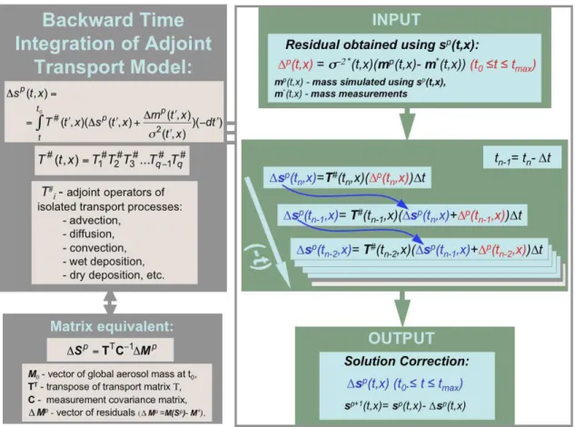
1Sˆp= ∇9m(Sp)=TTC−m11Mp, (40) where1Mp=M(Sp)−M∗, ∇9m(S) denotes the gradient of9m(S)andtpis a non-negative coefficient. This method uses the fact that the gradient∇9m(S)points in the direc-tion of maximal local changes of9m(S), and this direction (tp∇9m(Sp), generallytp<1) can always be used to correct Sp, so it moves toward the solutionS′that minimizes9m(S), i.e9m(Sp+1)<9m(Sp). Equations (39–40) do not require inversions of high dimension matrices (inverting a diagonal covariance matrix is trivial). The gradient∇9m(S)can be simulated using a time integration scheme similar to the one employed for forward modeling so the matrix solution of the steepest descent method Eqs. (39–40) can be replaced by an analogous continuous operation. Namely, the elements of the gradient vector∇9m(S)can be simulated in a manner simi-lar to Eqs. (2–4) and the inversion can be implemented using a continuous analog of the gradient vector∇9m(S)(see also Figs. 3–4). A continues equivalent of Eq. (40) can be written as follows (the detailed derivations is given in Appendix B):
1sˆp(t,x)=
t0
Z
t
T# t′,x
1sˆp t′,x
+σ−2 t′,x
1mp t′,x (−dt′),
(41a)
where
1mp(t,x)=m∗(t,x)−
t Z
t0
T t′,x m t′,x
+sp t′,x
dt′, (41b)
andT#(t,x)is the adjoint of the transport operatorT (t,x), that is composed of adjointsTi#(t,x)of the component pro-cessesTi(t,x):
T#(t,x)=T1#T2#T3#...Tq#−1Tq#. (41c) The vectors 1sˆp(t,x) and σ−2(t,x) 1mp(t,x) denote functional equivalents of vectors1SˆpandC−m11Mp respec-tively. For example, if one intends to use the continuous function1ˆsp(t,x)in numerical calculations, it can be rep-resented by a vector1Sˆpwith the following elements:
n 1Sˆpo
l =1ˆs p t
i, xj, yk, zm, (42a) where the index l is determined in the same way as in Eq. (34b).
Similarly, if the observational errors are uncorrelated, i.e. the covariance matrix of the measurementsCmis diagonal, with the diagonal elements equal toσ2 ti, xj, yk, zm
, the el-ements of vectorC−m11Mprelate to the continuous function
σ−2(t,x) 1mp(t,x)in straightforward way: n
C−m11Mpo l →σ
−2 t
i, xj, yk, zm
1mp ti, xj, yk, zm
. (42b) If observational errors do not have time correlations but do have spatial correlations,Cmhas an array structure that can be included in the algorithm (see Eqs. (B12–B15) in Ap-pendix B), provided one can formulate a weighting func-tionC−1(t,x,x′)from the covariance functionC(t,x,x′), to perform a role analogous to the one of matrix C−m1 in the discrete representation. Including the spatial correlations during each time moment is feasible because the model is integrated by time steps, and each step can be treated rather independently. However, accounting for observational errors that are correlated in time is not feasible without changing the structure of Eq. (41).
It is important to note that Eq. (41) is convenient for prac-tical implementation of the inversion. Indeed, as outlined in Fig. 4 (compare with Fig. 3), Eq. (41) is related to Eq. (4), with the difference that it uses1mp(t,x)in place ofs (t,x), and1ˆsp(t,x)in place ofm (t,x), and it performs the back-ward time integration of the adjoint operatorT#(t,x) . If T (t,x) is functionally equivalent to the matrix operatorT, then the adjoint operator T# (t, x) is an equivalent to the transposed matrix TT (Appendix A). Therefore, the main reason for developing the adjoint operator T# from T can be illustrated by considering matrix transposition. For ex-ample, since the transport operator integration can be ap-proximated using the split operator approach (e.g. see Ja-cob, 1999), where matrices corresponding to different atmo-spheric processes are multiplied at each time step (e.g. see Eq. 3). The following matrix identity is helpful:
(T3T2T1)T=(T1)T(T2)T(T3)T. (43) This reversing of the order of operations by transposition pro-duces an overturned sequence of component process applica-tions within each time step Eq. (41c), and reverses the order of integration in Eq. (41a), i.e. in backward time integration Eq. (41a). Also, the transposition of matrixTi changes rows and columns, so ifTis non-square, the input of (Ti)Tshould have the dimensions ofTi output, and vice versa. Thus, the adjoint model (Eq. 41) can be developed on the basis of the original model (Eq. 4) by reversing the order of operations and switching the inputs and outputs of the routines (e.g. El-bern et al., 1997; Menut et al., 2000).
Thus, using the adjoint of the transport model allows us to implement the LSM inversion (Eq. 9) without using ex-plicit matrix inversions, and therefore demands only moder-ate computational efforts. As is shown in Fig. 5 each iteration in Eq. (41) requires one forward integration of the transport model (Eq. 41b) followed by one backward integration of the adjoint transport model (Eq. 41a).
The need to perform a number of iterations in Eq. (41) is a potential drawback of implementing inversions via adjoint modeling. Indeed, the steepest descent method of Eqs. (39– 40), in general, converge to the exact solution after a very
large number of iterations. The even faster method of con-jugated gradients may require up toNS iterations (Press et al., 1992). Nevertheless, a rather limited number of simple iterations appears to be sufficient for global inverse model-ing of high dimensionality. For instance, the iterations of Eqs. (39–40) converge from an arbitrary initial guess to the solution rapidly if the following sequence tends toward the zero matrix (Dubovik, 2004):
∞ Y
p=1
I−tpTTC−m1T
⇒0, (44)
whereIis unity matrix. It is clear that rapid convergence of Eqs. (39–40) can be achieved only if TTT is predomi-nantly diagonal (Cm is often diagonal and does not cause problems). Fortunately, in transport modeling, the diago-nal elements ofTTTdominate, because local aerosol emis-sion typically influence only nearby locations (i.e. matrixT
is rather sparse and has a large number of zeros, see Eq. (B5) in Appendix B).
It should be noted that Eqs. (41) expressing the inver-sion via adjoint operators, are generally analogous to tech-niques used in variational assimilation (e.g. Le Dimet and Talagrand, 1986; Talagrand and Courtier, 1987; Menut et al., 2000; Vukicevic et al., 2001). Nevertheless, the statistical es-timation approach employed in our study makes it possible to establish direct relationships between Eqs. (41) and conven-tional LSM minimization which therefore improves flexibil-ity in implementing the inversion. For example, using error covariances directly makes it possible to account for differ-ent levels of accuracy in the inverted observations. Moreover, formulating the inversion using a statistical approach is con-venient for including several a priori constraints in the same retrieval, for example, by following multi-term LSM strategy discussed in Sect. 2.4.
2.6 Including a priori constraints in inversion, using adjoint equations
Equations (41) can be easily adopted for constrained inver-sion. Figures 6–7 illustrate the considerations discussed in this Section. For example, the inversion constraining the so-lution Sˆ with its a priori estimates S∗, shown as a matrix inversion in Eq. (13), can be implemented iteratively, e.g. us-ing steepest descent iterations:
ˆ
Sp+1=Sˆp− tp1Sˆp, (45a)
1Sˆp=∇9m(Sp)+∇9S(Sp)=TTW−m11F p+γ
sW−s11S p.
(45b) Here we used weighting matricesW...instead of covariance matricesC... in order to align these equations with the LSM multi-term formulations given by Eqs. (28–32). If we assume
9
Fig. 6.illustrating implementation of the steepest descent method with a priori constraints, by means of adjoint aerosol transport modeling.
for simplicity that all measurements are statistically indepen-dent and have the same accuracyεm(i.e.Cm=Iε2m→Wm=I), and that all a priori estimates are statistically independent and have the same accuracyεs (CS=Iε2S→WS=I), then we can write the continuous analog to Eq. (45b) as follows:
1ˆsp(t,x)= t0
Z
t
T# t′,x
1ˆsp t′,x
+1mp t′,x (−dt′)
+γS sˆp t′,x−ˆs∗ t′,x. (45c) whereγS=ε2m/ε2S.
The iterative analog to Eq. (35), constraining the solution by limiting the time and spatial derivatives ofS (t,ˆ x), can be written as follows:
ˆ
Sp+1=Sˆp−tp1Sˆp, (46a)
1Sˆp= ∇9m(Sp)+ X
(q=t,x,y,z)
γq∇9q(Sp)
=TTW−m11Fp+ X (q=t,x,y,z)
γqDTnDnSp. (46b)
The function 1ˆsp(t,x), corresponding to vector 1Sˆp can be formulated as follows:
1ˆsp(t,x) = t0
Z
t
T∗(t,x) 1ˆsp t′,x
+1mp t′,x (−dt′)
+ X
(q=t,x,y,z)
γqD#nDnsp(t,x)=
= t0
Z
t
T∗(t,x) 1ˆsp(t′,x)+1mp(t′,x)(−dt′)
+ X
(q=t,x,y,z) γq
∂(2n)sp(t,x)
∂q(2n) , (47)
wherex′=(xj, yk, zm),Dn denotesn-th derivative operator andDn# denotes the adjoint to then-th derivative operator. For the adjoint operatorDn#, one can write the following:
D#n=(−1)nDn. (48a)
80
Fig. 7.Illustration of the combination of sequential backward time integration of the adjoint aerosol transport model with a priori constraints.
This identity can be obtained from the transposition of the matricesDn. For example, forD1Twe have the following:
DT1 =
1 −1 0 . . . 0 1 −1 0 . . . 0 0 1 −1 0 . . . . . . . . . . 1 −1 0 . . . 0 1 −1
T
=
1 0 . . . −1 1 0 . . .
0 −1 1 0 . . . . . . . . . . .−1 1 0 . . . 0 −1
. (48b)
Here one can see that with exception of the first and last lines ofD1T, each row corresponds to first differences.
Sim-ilarly, it is easy to demonstrate that the lines of the matrices
DnT(n >1) corespond ton-th differences, with exception of first and lastnlines. If both the number of lines and columns inDnT are much larger thann, this difference betweenDn andDnTcan be neglected, e.g. in the continuous case when 1q−>0. For example, when the norm of the second deriva-tives of s(t,x)over time is constrained, the following
re-lationship can written for the p-th element of the gradient ∇9t(Sp):
D#2D2Sp(t,x)|ti =
∂4Sp(t,x) ∂t4
ti
≈ {9t(Sp)}g=
=(1t )−4(S(ti+2,x)−4S(ti+1,x)+6S(ti,x)
−4S(ti−1,x)+S(ti−2,x)) (49)
where the indexgcan be calculated according Eq. (34) and 2<i<Nt–2 (see Eq. 21). Equations analogous to Eq. (49) can be written for terms corresponding to the spatial coordinates x,yandz. It should be noted that in practice, the calculation of the first “transport term” and the second “a priori term” in Eq. (47) can be performed rather independently as shown in Fig. 6. For example, in Section 3 (where Eq. (47) is imple-mented) the “transport term” is integrated with the time step of the GOCART model (20 min), whereas the “a priori term” is calculated as shown in Eq. (49) with time step1t=ti+1−ti equal to 24 h.
These formulations can also adopt the same a priori con-straints as those used in the Kalman filter, i.e. when only the continuity of sources is constrained a priori by assum-ing S∗t=St−1+1S (see Eqs. 15 and 18). In this situation, one can assume that the first derivative ofs(t,x)over time is
used with only one a priori term, corresponding to the norm of the first derivatives∂s(t,x)/∂ti.e.q=tandn=1. This way Eq. (47) relies on the same a priori constraints as those used in the Kalman filter Eq. (47), and observationsm(t,x) dur-ing the entire time period t >ti can contribute to the solu-tion S(ti,x), whereas Eq. (15) relies only on observations m(ti,x)at timeti.
Also, it should be noted that for clarity Eqs. (45c) and (47) were written for the case of the simplest measurements co-variance matrices and a priori data errorsC...=ε2...I.... How-ever, the generalization of these equations to cases when the accuracies within each data set are different ({C}ii6={C}jj, i6=j), or the covariance matrices are non-diagonal, is rather straightforward (similar to that shown by Eqs. (41–43). 2.7 Inverting models having non-linearities
Previous sections described an approach to inverting a linear transport model (Eq. (5)), provided global aerosol massM∗ measurements are available. In practice, the transport model may be non-linear, and the global aerosol data fields may be available only in the form of satellite optical measurements:
f =F (m(t,x), λ, θ;...), (50)
wheref(. . . ) is generally a non-linear function depending on aerosol massm(t,x), instrument spectral characteristicsλ, observation geometryθ, etc. Therefore, the following non-linear equation should be solved instead of Eq. (5):
F∗=F(M(S))+1F, (51)
whereF and1F are vectors of global optical data and their uncertainties. Since, the steepest descent method can be ap-plied to both linear and non-linear problems, Eqs. (41, 45, 47), that use adjoint operators, can be expanded to solve Eq. (51). For example, for a basic case when only optical measurementsF∗ are inverted with no a priori constraints, the steepest descent solution can be written as:
ˆ
Sp+1=Sˆp−tp1Sˆp, (52a)
1Sˆp = ∇9f(Sp)=KTpC− 1 f 1F
p=TT pFTpC−
1 f 1F
p,(52b) where1Fp=F(Sp)–F∗. MatricesKpTpandFpdenote Ja-cobi matrices of the first derivativesdf/ds, dm/ds anddf/dm calculated in the vicinity of the vectorSp:
Kp j i=
dfj(m(S), λ, θ, ...) dSi
S=Sp
, (53a)
and
Tp j′i =
dmj′(S, t,x)
dSi S=Sp
,
Fp j i′ =
dfj(M, λ, θ, ...) ∂mi′
Mp=M(Sp)
, (53b)
ments j j, i, i of the corresponding vectors F = (f1,f2,. . . ), MT=(m1,m2,. . . ), andST=(S1,S2,. . . ). The
fol-lowing relationship between the Jacobi matrices of df/ds, dm/dsand thedf/dmderivatives was used in Eq. (53):
Kp=FpTp . (53c)
The function1ˆsp(t,x), corresponding to vector1Sˆp, can formulated as follows:
1ˆsp(t,x)= t0
Z
t
Tp# t′,x
Fp# t′,x
1ˆsp t′,x
+1fp t′,x
(−dt′), (54)
where Tp#(t,x) and Fp#(t,x) are adjoint operators for the mass transportT (s(t,x))and the optical modelF (m(t,x)), and indexpindicates that these adjoint operators are equiv-alents of transposed Jacobi matricesTTpandFTp. The deriva-tion ofFp#(t,x)is quite transparent because optical proper-tiesf (m(t,x), . . . ) usually are related only to local aerosols, so in practical implementations of Eq. (54) (that are usually performed in discrete representations), Fp#(t,x)can be ex-plicitly replaced by the transposed Jacobi matrixFTp.
Equation (54) can be expanded easily to implement a con-strainted inversion off=F (m(t,x), λ, θ, ...). For example, when the solution is constrained by a priori limits on the tem-poral and spatial derivatives ofS (t,ˆ x)(utilized in Eqs. 35 and 48), Eq. (54) can be written as follows:
1sˆp(t,x)=
t0
Z
t
Tp# t′,x
Fp# t′,x
1sˆp t′,x
+1fp t′,x (−dt′)
+ X
(q=t,x,y,z) γq
∂q(2n)
(sp(t,x)) ∂q(2n). (55)
Using this1ˆsp(t,x), (if the same discrete representation is used), the iterative retrieval would amount to minimizing the following quadratic form:
29(S)=29f(S)+2 X
(q=t,x,y,z)
γq9q(S)=
2(1F)T 1F+2 X (q=t,x,y,z)
γqSTDTn,qDn,qS. (56a)
This quadratic form can be generalized by the following functional:
29′=2 Z
t Z Z Z
x,y,z
1f#(t, x, y, z) 1f (t, x, y, z)dxdydzdt
+2 X (q=t,x,y,z)
γq qmax
Z
qmin
∂ns(q, ...)
∂qn 2
dq, (56b)
where1f (t, x, y, z)=f∗−f (t, x, y, z)and1f#(t, x, y, z) denotes the adjoint of1f (t, x, y, z).
Thus, the above derivations show the high potential of using a statistical estimation approach for implementing aerosol transport inverse modeling. For example, it was demonstrated that by following the multi-term LSM strat-egy, there is flexibility to apply various types of a priori constraints in inverse modeling. For example, Eqs. (46–49) show how constraints on aerosol (or other tracer) emission derivatives with respect to spatial coordinates or time can be included in the adjoint integration of tracer models, that are widely used in variational assimilation for atmospheric tracer source identification (e.g. Le Dimet and Talagrand, 1986; Ta-lagrand and Courtier, 1987). Using such constraints in in-verse modeling may have high potential because, in princi-ple, a priori limitations on the derivatives of emission vari-ability is a weaker and more flexible way of constraining the solution than assuming a priori values of the emission. Equa-tions (55–56) give the formulation of the approach for invert-ing satellite observations (e.g. radiances measured by pas-sive satellite observations). This generalization may have the high potential, because using satellite observations directly in inverse modeling and satellite data assimilation has ad-vantages compared to relaying on satellite retrieval products (Weiver et al., 2006). However, using the steepest descent iteration in Eqs. (55–56) makes the application of Eqs. (55– 56) less attractive in practice, because generally, inverting ra-diative transfer equations by the method of steepest descent requires a large number of iterations (Dubovik and King, 2000). Therefore, it might be useful to explore the possibil-ity of adopting iterative strategy of the conjugated gradients method (Appendix C), as this method is known to have su-perior convergence properties than steepest descent.
3 Application of the inverse methodology for aerosol source retrieval from satellite observations
– First, we consider the inversion of an aerosol transport model, to derive the “unknown input” (aerosol emis-sions) to the model from the “known output” (aerosol mass distribution). Our inverse algorithm developments are based on the GOCART aerosol transport model.
– Second, we discuss differences between inverting the model output and satellite data and outline the modifi-cations required for applying the model based inverse algorithm to the satellite observations. We consider in-version of the aerosol observations from MODIS.
– Finally, we illustrate the performance of developed al-gorithm by numerical tests and then we apply the algo-rithm to the actual MODIS aerosol data.
3.1 Algorithm for inverting the GOCART model
The inversion algorithm (Eqs. 39–41) treats the strength of the aerosol emission at each global location as an unknown.
Therefore, in an ideal situation, when the observations pro-vide enough information to retrieve all the emission pa-rameters, the emissions derived from the observations the-oretically could replace the original module prescribing the aerosol emissions in the chemical transport model. Such an ideal situation is likely if reliable observations about all the aerosol characteristics are provided by the transport model output, i.e. if these observations are sensitive to all the time and space (4D) aerosol variations provided by model. As we will discuss in the next Section, the real observations are not sensitive to all the aerosol distribution details that can be modeled, therefore successful inversion of model output does not guarantee the successful inversion of real observa-tions. Nonetheless, inverting the detailed model output can be helpful for verifying the performance of different blocks in the inversion algorithm. As a first step in implementing the inverse algorithm, we developed an algorithm to invert GOCART output, and carried out series of numerical tests to verify algorithm performance under highly constrained con-ditions (the entire output is prescribed) and in a “no error” environment.
The GOCART – Goddard Chemistry Aerosol Radiation and Transport model is described in papers by Chin et al., (2000, 2002) and Ginoux et al. (2001). The model uses the assimilated meteorological data from the Goddard Earth Observing System Data Assimilation System (GEOS DAS) and provides four-dimensional aerosol mass distributions in 20 to 30 atmospheric layers, at a horizontal resolution of 2◦latitude by 2.5◦longitude. The model calculates aerosol composition and size distribution, optical thickness and ra-diative forcing. There are seven modules representing at-mospheric processes: emission, chemistry, advection, cloud convection, diffusion (boundary layer turbulent mixing), dry deposition, and wet deposition. The model solves the conti-nuity Eq. (1) using an operator-splitting technique (Eqs. 2– 3), with a time step of 15 min for advection, convection and diffusion, and 60 min for the other processes.
GOCART provides 4D distributions of about 16 aerosol particle types/size bins: sulfate, hydrophilic and hydrophobic Organic Carbon (OC), hydrophilic and hydrophobic Black Carbon (BC), four size-differentiated sea salt bins, and up to seven dust size-differentiated bins, depending on the GO-CART model version (Chin et al., 2002, 2004; Ginoux et al., 2001). The model does not include interactions between different aerosol particles, with the exception of transforma-tions between hydrophilic and hydrophobic components of BC and OC. Therefore, GOCART simulates distributions of sulfates, BC, OC, desert dust and sea salt independently. Cal-culations for different size bins of dust and sea salt are also independent, and the atmospheric processes sensitive to par-ticle size (e.g. sedimentation) are incorporated accordingly. The same concept can be adopted for inverting the model out-put, i.e. each aerosol component of the output can be inverted independently with an inverse algorithm that uses an adjoint model tuned to the properties of each aerosol component.
and 55) and illustrated by diagrams in Figs. 5 and 6 was implemented for the GOCART model. The adjoint trans-port operatorT∗p(t,x)was developed by redesigning GO-CART modules for each atmospheric process. Namely, the adjoint operation for advection was performed with the orig-inal GOCART advection algorithm (Lin and Rood, 1996), using sign-reversed wind fields (Vukicevic et al., 2001). The equivalence between such physically derived retro-transport and adjoint equations has been proven rigorously by Hour-din and Talagrand (2006). The adjoints of the local pro-cesses were developed by analogy with the corresponding transpose matrix operators. Specifically, cloud convection, diffusion, dry deposition, and wet deposition affect only ver-tical aerosol motion. All these processes have local char-acter in the sense that for a single time step in the model, they work independently in each horizontally resolved ver-tical column. Therefore, such processes can be easily mod-eled via explicit use of matrices of rather small dimension, and the corresponding adjoint operators can be obtained by direct transposition of those matrices. First, we arranged the cloud convection, diffusion, dry deposition, and wet deposi-tion in matrix form, and derived the transpose of those ma-trices. Then, for achieving faster calculation time, we re-designed the original programs so that their application to a vector provides a product equivalent to the application of the corresponding transpose matrices. Chemical aging transfor-mations of black and organic carbon aerosols require chang-ing only the proportions of different components, and do not induce any vertical or horizontal aerosol motions. Therefore, the adjoints of these chemical processes can be constructed simply by changing the direction of chemical transformation. Once the adjoint model was developed, we implemented sev-eral inversions of 4D mass fields simulated by GOCART for different aerosol components. These numerical tests showed that the algorithm retrieves the emissions of all aerosols ac-curately and no inversion issues that could substantially limit the accuracy of the aerosol source retrievals in such well-constrained situations were revealed. Particular emphasis was placed on testing inversions of BC, OC and dust, since we expect algorithm applications to be focused on observa-tions of these types of aerosol.
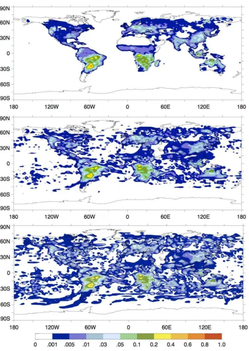
3.2 Application of the algorithm for inverting satellite data Naturally, satellite observations (as well as observations of any other type) do not provide the same aerosol quantities, coverage, and sampling as model simulations (see Fig. 8). Accordingly, the inverse algorithm settings, as well as some aspects of inversion concept, needs to be adjusted when in-verting observations. Below we discuss in detail the appli-cation of inverse modeling for retriving global aerosol emis-sions from MODIS data, though many of the aspects consid-ered are relevant to inverse modeling with any other satellite data.
diometer aboard both NASA’s Terra and Aqua satellites, pro-vides near-global daily observations of Earth over a wide spectral range (0.41 to 15.0µm). These measurements are used to derive spectral aerosol optical thickness and aerosol size parameters over land and ocean (Kaufman et al., 1997; Tanr´e et al., 1997; Remer et al., 2005). The primary aerosol products avaiable include aerosol optical thickness at three visible wavelengths over land and seven wavelengths over ocean, aerosol effective radius, and fraction of optical thick-ness attributed to the fine mode. The present study uses the MODIS aerosol optical thickness product aggregated to 1◦ by 1◦spatial resolution. The expected accuracy of MODIS optical thickness is1τ=±0.03±0.05τ over ocean (Tanr´e et al., 1997; Remer et al., 2005) and1τ=±0.05±0.15τ over land (Kaufman et al., 1997; Remer et al., 2005).
3.2.1 Main issues for applying inverse modeling to the MODIS data
First, to use MODIS observations as input to the inversion, the adjoint formulation must include the conversion from modeled aerosol mass into measured aerosol optical param-eters. Accordingly, the operator Fp is rearranged into the adjointFp#and is used in the inversion according to Eqs. (54– 55). Since the aerosol optical thickness operatorFpsums the contributions from different layers and aerosol types, its ad-joint Fp# redistributes the total sum to the individual layers and aerosol types.
Second, the MODIS globalτ(0.55) observations reported at 1◦by 1◦need to be rescaled to the 2◦by 2.5◦GOCART horizontal resolution.
Third, as mentioned above, satellite data provide less in-formation than global model output. Specifically, a passive, multi-spectral, polar-orbiting, cross-track scanning, single view remote sensor such as MODIS has the following main limitations (Kaufman et al., 1997; Tanr´e et al., 1996, 1997; Remer et al., 2005).:
– no sensitivity to aerosol vertical distribution;
– global coverage only once in two days, only for cloud-free conditions, and not over bright surfaces such as deserts or in glint regions over water;
– limited capability to identify aerosol type based on coarse/fine mode size discrimination only; no informa-tion about particle shape or composiinforma-tion.
Indeed, the top-of-atmosphere radiances are sensitive mainly to the total effective aerosol content in the atmo-spheric column. But it is worth noting that coarse/fine mode discrimination contains some particle type information, as desert dust and maritime aerosols are dominated by coarse mode particles, whereas biomass burning and urban pollu-tion are dominated by fine mode particles (Dubovik et al., 2002). In summary, the problem of retrieving all the aerosol