www.atmos-meas-tech.net/5/1823/2012/ doi:10.5194/amt-5-1823-2012
© Author(s) 2012. CC Attribution 3.0 License.
Measurement
Techniques
Retrieving aerosol in a cloudy environment: aerosol product
availability as a function of spatial resolution
L. A. Remer1, S. Mattoo2,3, R. C. Levy2,3, A. Heidinger4, R. B. Pierce4, and M. Chin2
1Joint Center for Earth Systems Technology, University of Maryland Baltimore County, Baltimore MD 21228, USA 2Earth Science Division, NASA Goddard Space Flight Center, Greenbelt MD 20771, USA
3Science Systems and Applications, Inc., Lanhan MD 20709, USA
4Center for Satellite Applications and Research, NOAA at the Cooperative Institute of Meteorological Satellite Studies
(CIMSS), University of Wisconsin, Madison WI, USA
Correspondence to: S. Mattoo ([email protected])
Received: 27 December 2011 – Published in Atmos. Meas. Tech. Discuss.: 13 January 2012 Revised: 4 June 2012 – Accepted: 3 July 2012 – Published: 30 July 2012
Abstract. The challenge of using satellite observations to re-trieve aerosol properties in a cloudy environment is to pre-vent contamination of the aerosol signal from clouds, while maintaining sufficient aerosol product yield to satisfy spe-cific applications. We investigate aerosol retrieval availabil-ity at different instrument pixel resolutions using the standard MODIS aerosol cloud mask applied to MODIS data and sup-plemented with a new GOES-R cloud mask applied to GOES data for a domain covering North America and surround-ing oceans. Aerosol product availability is not the same as the cloud free fraction and takes into account the techniques used in the MODIS algorithm to avoid clouds, reduce noise and maintain sufficient numbers of aerosol retrievals. The in-herent spatial resolution of each instrument, 0.5×0.5 km for MODIS and 1×1 km for GOES, is systematically degraded to 1×1, 2×2, 1×4, 4×4 and 8×8 km resolutions and then analyzed as to how that degradation would affect the avail-ability of an aerosol retrieval, assuming an aerosol product resolution at 8×8 km. The analysis is repeated, separately, for near-nadir pixels and those at larger view angles to inves-tigate the effect of pixel growth at oblique angles on aerosol retrieval availability. The results show that as nominal pixel size increases, availability decreases until at 8×8 km 70 % to 85 % of the retrievals available at 0.5 km, nadir, have been lost. The effect at oblique angles is to further decrease avail-ability over land but increase availavail-ability over ocean, because sun glint is found at near-nadir view angles. Finer resolu-tion sensors (i.e., 1×1, 2×2 or even 1×4 km) will retrieve aerosols in partly cloudy scenes significantly more often than
sensors with nadir views of 4×4 km or coarser. Large dif-ferences in the results of the two cloud masks designed for MODIS aerosol and GOES cloud products strongly reinforce that cloud masks must be developed with specific purposes in mind and that a generic cloud mask applied to an indepen-dent aerosol retrieval will likely fail.
1 Introduction
agencies and communities in mitigating and warning popu-lations of potential dangers (Al-Saadi et al., 2005).
Both climate and air quality applications require contin-ual monitoring of aerosol loading over broad geographical regions. For climate, a global perspective is needed (Kauf-man et al., 2002; Remer et al., 2009). For air quality, even if interest is more regional, there is need for a more complete coverage and higher density of spatial sampling than a net-work of ground-based in situ monitoring stations can provide (Chu et al., 2003; Prados et al., 2007; Gupta and Christo-pher, 2009). Both these applications are increasingly relying on satellite retrievals of aerosol information to provide the observational constraints on models, offer new insights on aerosol distributions, and provide day-to-day coverage and accumulated statistics of aerosol properties (Stier et al., 2005; Yu et al., 2006; van Donkelaar et al., 2006, 2011). Satellites make a unique contribution to climate and air quality studies by providing the global coverage needed for climate applica-tions and the density of coverage needed by the air quality community.
Aerosol properties can be derived from space-based ob-servations with well-defined uncertainties, and used success-fully in a wide array of applications (Remer et al., 2005; Kahn et al., 2010; Torres et al., 2007; Tanr´e et al., 2011). However, making aerosol retrievals on an operational ba-sis is difficult, and making aerosol retrievals in cloudy en-vironments is especially difficult (Zhang et al., 2005; Wen et al., 2006; Marshak et al., 2008). Aerosol retrievals in a cloudy environment require that a “cloud mask” be devel-oped that separates cloudy from cloud-free scenes (Martins et al., 2002). Traditionally aerosol has only been derived in cloud-free scenes, although efforts are underway to derive aerosol above clouds using certain sensors (Jethva and Tor-res, 2011; Waquet et al., 2009, 2010). Separating clouds and aerosols is inherently difficult because there exists no clearly defined separation between the two in any variable. This is an issue of measurement systems, but also an inherent physical continuum between aerosol particles, wet aerosol particles, activated cloud droplets and dissipated cloud fragments (Ko-ren et al., 2007; Charlson et al., 2007). Remote sensing algo-rithms employ complicated schemes, using many variables (Ackerman et al., 1998; Frey et al., 2008), to make this sep-aration as best they can, but no “cloud mask” is perfect. The reality is that different cloud masks are produced for different purposes.
A cloud mask designed for an aerosol retrieval, ideally, must exclude all cloud and cloud remnants from a pixel des-ignated as “cloud-free”. On the other hand, extreme restric-tion that avoids any cloud contaminarestric-tion would prevent a sufficient number of aerosol retrievals from being made for a specific application. Thus, there is a tradeoff between per-fect protection of the aerosol product and availability of that product, as some pixels must be designated “cloud-free” in order for an aerosol product to be obtained. The degree of the accuracy and availability of retrieved aerosol products
criti-cally depends on the cloud mask criteria and the instrument’s pixel resolution.
Here, we explore the availability of an aerosol retrieval in a cloudy environment.Availability is defined as the number of product boxes available for aerosol retrieval divided by the total number of boxes in the region or time period of in-terest. A product box contains one aerosol retrieval, and the size of the product box may be larger than the inherent pixel size of the instrument. First, we demonstrate the concept that different cloud masks are defined for different purposes. Sec-ond, we provide details of the MODerate resolution Imag-ing Spectroradiometer (MODIS) aerosol cloud mask and a second cloud mask developed for the Geostationary Opera-tional Environmental Satellite-R (GOES-R) data, and explain the different purposes of the two cloud masks. Third, using the MODIS cloud mask, we examine the availability of an aerosol retrieval over North America and surrounding oceans under varying pixel spatial resolutions, and investigate possi-ble differences between near-nadir views and oblique angles. We supplement the MODIS analysis by applying a similar procedure to one day of the GOES-R cloud mask to explore the possibility of a geosynchronous satellite to resolve day-time variations of aerosols at different sensor pixel resolu-tions. In the end we discuss the implications of these results to currently proposed satellite missions.
2 MODIS and GOES
The twin MODerate resolution Imaging Spectroradiometers (MODIS) were launched aboard NASA’s Terra and Aqua polar orbiting satellites in December 1999 and May 2002, respectively. MODIS has 36 channels spanning the spectral range from 0.41 to 15 µm, and representing three spatial res-olutions: 250 m (2 channels), 500 m (5 channels), and 1 km (29 channels). The aerosol retrieval makes use of eight of these channels (0.41–2.13 µm) to retrieve aerosol character-istics, and uses additional wavelengths in other parts of the spectrum to identify clouds and river sediments. No aerosol retrievals will be analyzed in this study, only the cloud mask produced by the MODIS aerosol algorithm. MODIS scans cross track, observing each target at only one angle per orbit. Swath width is 2330 km, which provides at least one view of almost every target on the Earth each day, and multiple daily views of high latitude locations.
longitude and the same latitude, is scanned in 26 min or less. Scans of just North America or the continental United States are much faster. GOES produces an aerosol product (Prados et al., 2007), but these will not be analyzed in this study. Only the cloud mask developed for GOES-R, which has not yet been launched, will be applied to GOES data and used in this study. This cloud mask is described in the next section.
3 Cloud masks
The term “cloud mask” is a common term used by the satel-lite remote sensing community, but it has three separate con-notations depending on its intended purpose. There are cloud masks developed to identify clouds, those to protect a re-trieval of surface properties and, finally, those designed to protect an aerosol retrieval. All of them identify clouds, but each makes decisions in how to define a cloud or cloud-free scene that best suits the ultimate goal of the remote sensing algorithm.
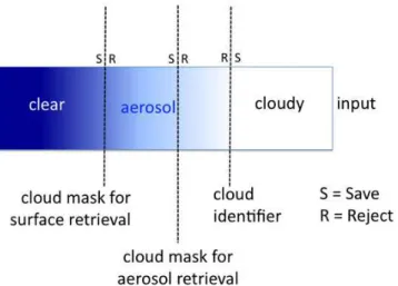
For example, a cloud mask that selects pixels for retrieval of cloud properties is going to select the cases best suited for a retrieval of cloud properties. Marginal cloud edges, cloud fragments and pixels that are not overcast will be designated “cloud free” by this type of cloud mask. On the other hand, a cloud mask whose purpose is to select cloud free pixels for retrievals of surface properties will take the entirely opposite approach. Those pixels containing marginal cloud edges and fragments designated by the first cloud mask as “cloud free” will be assigned “cloudy” in the surface retrieval algorithm. In addition, the surface retrieval algorithm will also not take a chance when the scene is obscured by aerosol. If the scene is obscured by either cloud or by heavy aerosol, the pixel will be designated “cloudy”. Clearly, both cloud masks are not suitable for aerosol retrieval, as the first one will introduce significant cloud contamination in aerosol products and the second one will prevent retrieving heavy aerosol loadings. Therefore, an aerosol algorithm has to be designed that elim-inates marginal cloud situations and still designates the heavy aerosol events as “cloud free”. Figure 1 illustrates the posi-tioning of potential thresholds along a gradient of satellite-measured inputs representing the deep blue ocean surface overlaid by a gradual increase of aerosol and then cloud par-ticles.
Figure 2 shows an example of three different cloud masks applied to the same MODIS image in a situation where heavy aerosol coincides with a cloud field. These cloud masks are listed in Table 1. The standard cloud mask (Ackerman et al., 1998; Frey et al., 2008) applied to the image and shown in the upper right panel does not attempt the retrieval of heavy dust aerosols overlaying the cumulus field. It desig-nates almost the entire left third of the image as “cloudy”. This cloud mask corresponds to the “cloud mask for sur-face retrieval” of Fig. 1. Meanwhile the algorithm producing cloud optical thickness (Platnick et al., 2003), shown in the
Fig. 1. Schematic illustrating thresholds of input used to differen-tiate clear from cloudy for different purposes. For the purpose of a surface retrieval, only the clearest pixels are saved. For the pur-pose of a cloud identifier, only the cloudiest pixels are saved. For the purpose of an aerosol retrieval, a mid-range threshold must be determined.
lower left panel, is much choosier, selecting many fewer pix-els for a cloud retrieval than was designated “cloudy” by the first cloud mask. The lower left panel is an example of the “cloud identifier” of Fig. 1. The aerosol cloud mask (Martins et al., 2002) used to make an aerosol retrieval is also dif-ferent than the first cloud mask. In the upper left corner of the image, the aerosol cloud mask avoids some of the pixels that the first cloud mask designated as “cloud free”, and yet finds holes in the cloud field on the left side of the image to perform an aerosol retrieval. It also designates the area cov-ered by dust as “clear” to allow aerosol retrieval, in contrast with the standard cloud mask. The aerosol cloud mask is not created simply by drawing the threshold between the other two cloud masks, as is suggested by the one-dimensional schematic in Fig. 1. There are several variables under con-sideration, and the result is a cloud mask that is both more and less conservative than the mask designed for surface re-trieval. Note also that the aerosol cloud mask is not the simple inverse of the cloud identifier for the cloud optical thickness retrieval.
The main point is that a cloud mask must be designed with a specific retrieval in mind. A one-size-fits-all cloud mask will not succeed.
4 MODIS and GOES-R cloud masks
Fig. 2. Terra MODIS image from 12:00 UTC 2 July 2010 showing (upper left) true color image of heavy dust spreading over the At-lantic from northern Africa. (Upper right) standard MODIS cloud mask (MOD35) with white areas identified as cloudy, gray as sun glint, red as probably cloudy, blue probably clear and green as clear. (Lower left) MODIS cloud optical thickness product (MOD06), and (lower right) MODIS aerosol cloud mask (MOD04) with white des-ignating cloudy and blue, cloud-free. This panel shows only the cloud mask, not the pixels chosen for aerosol retrieval. Aerosol re-trievals are not made in the sun glint region. The red oval identifies a region where the aerosol cloud mask finds more clouds than the standard cloud mask. The red arrow identifies an area that neither the cloud retrieval nor the aerosol retrieval chooses to use to derive cloud or aerosol properties, respectively.
4.1 MODIS aerosol cloud mask
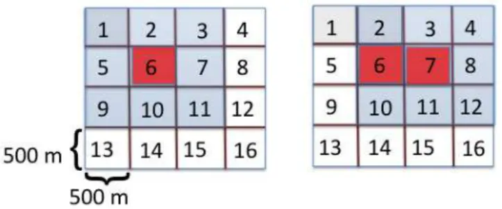
The purpose of the MODIS aerosol cloud mask is to protect the products of the MODIS aerosol retrieval algorithm from cloud effects while maintaining adequate product availabil-ity at all levels of aerosol loading. The cloud mask must be able to separate heavy aerosol events from clouds. The ba-sis of the retrieval is spatial variability. Sets of 3×3 0.5 km resolution reflectance values are examined and standard de-viation is calculated from the 9 pixels. Throughout this work pixel resolution is a nominal value, defined at nadir. Pixels in the MODIS image actually increase in size as view angle in-creases and the view becomes more oblique. A 0.5 km pixel at nadir will increase in area by a factor of 4 to become a 2 km pixel at swath edge. The spatial resolution test described here uses sets of 3×3 pixels, which are composed of 0.5 km pixels at nadir and 2 km pixels at the edges. If the standard deviation of the reflectance of the 9 pixels, no matter their actual size, exceeds a designated value, at least one of the pixels must be cloudy. The single, nominal 0.5 km pixel in the center is designated “cloudy” and the window of 3×3 pixels moves one column over to the right. The standard deviation test is repeated along the entire span of the image, then advanced by one 0.5 km pixel in the along track image (down) and
contin-ued. The procedure is repeated until all pixels in the image have been tested. Figure 3 illustrates this technique. The ad-vancing 3×3 window will overestimate cloudiness to some degree, because if the cloudy pixel in the Fig. 3 example is pixel 5, the spatial variability test will also mask out pixels 1, 2, 6, 9 and 10, and the contiguous pixels to the left if this did not represent the edge of the scan. The goal is to be suffi-ciently conservative to remove some of the pixels contiguous to the actual cloudy pixel.
In the MODIS over ocean retrieval, the spatial variability test is applied using reflectance at 0.66 µm to avoid ocean color variability. In the over land retrieval, the algorithm ap-plies the spatial variability test to the 0.47 µm channel be-cause the land is darker at this wavelength. The algorithms also apply a similar spatial variability test to the 1.38 µm channel using 1 km pixels, because this channel is particu-larly sensitive to thin cirrus. Over ocean, additional tests us-ing absolute reflectance at 1.38 µm and the ratio of the flectances of the 1.38 and 1.24 µm channels attempt to re-move further effects of thin cirrus (Gao et al., 2002). Finally, there are three cloud mask tests using the longwave chan-nels at 1 km that are adapted from the standard MODIS cloud mask (MOD/MYD35). These are the infrared thin cirrus test (Bit 11), the 6.7 µm test for high cloud (Bit 15) and the split window test (Bit 18) (Ackerman et al., 2010). All of these tests must return a “cloud free” designation for the 0.5 km pixel to be further considered for an aerosol retrieval. In the case of a test applied to 1 km reflectances, a “cloudy” des-ignation at 1 km will be passed to all 4 of the 0.5 km pixels affected. The binary, “cloudy”/“cloud free”, designations at 0.5 km are reported in the MODIS Collection 6 product as Aerosol Cldmask Land Ocean.
Fig. 3. Illustration of MODIS aerosol cloud mask spatial variabil-ity test. The algorithm identifies a set of 3×3 0.5 km pixels and calculates standard deviation of the reflectance of those 9 pixels. If the standard deviation exceeds a designated value, the center pixel (pixel 6) is designated “cloudy” (denoted by shaded red in the fig-ure). Then the algorithm moves one column to the right and tests the next set of 3×3 pixels to determine if pixel 7 is “cloudy”.
the brightest and darkest pixels. The arbitrary discarding of bright and dark pixels removes residual cloud and surface features and cloud shadows that are not otherwise addressed. The ocean algorithm requires a minimum of 10 remaining pixels to make a retrieval for a 10×10 km aerosol product. The land algorithm requires 12.
Figure 4 also illustrates the point that the nominal instru-ment pixel resolution (0.5 km) is not necessarily the same as the aerosol product resolution (10 km), and that product res-olution boxes do not need to be entirely cloud free in order to retrieve an uncontaminated aerosol product. Creating a prod-uct resolution coarser than the resolution of the input pixel reflectance allows much discretion in selecting pixels for re-trieval while maintaining high levels of product availability.
4.2 GOES-R cloud mask
The GOES-R Algorithm Working Group Cloud Mask (ACM) is a cloud identification algorithm as defined in Fig. 1. It was developed for the Advanced Baseline Imager (ABI) that will fly on GOES-R, which will provide 16 spec-tral observations with a spatial resolution of 2 km for the IR channels and 0.5 km for the visible (0.65 micron) channel. The ACM uses 15 tests to detect the presence of cloud. Of these 15 tests, 11 use IR channels and 4 use solar reflectance channels. Four of the ACM tests exploit spatial heterogene-ity to detect cloud and two exploit temporal information. The ACM returns 4 levels of cloudiness (clear, probably-clear, probably-cloudy and cloudy). Any positive test for cloud re-sults in a cloudy classification. Cloud pixels that border a non-cloudy pixel are reclassified as probably-cloudy. Clear pixels that fail one or both of two spatial uniformity tests are classified as probably-clear. The ACM provides the results of each test. The goal of the ACM was to provide other GOES-R Algorithm Working Group algorithms useful information on cloudiness and the flexibility to optimize the cloud mask for their applications. In this paper, both clear and
probably-clear results were used to compute GOES-R aerosol avail-ability values shown later.
The thresholds for the ACM tests were computed using 4 months of collocated CALIPSO/CALIOP and MSG/SEVIRI data. The thresholds were set so that the false alarm rates from each test were under 2 %. A false alarm is when a pixel is identified as a cloud, but is not. The overall goal of the ACM was to minimize false alarm rates at the risk of increased rates of missing clouds. The guidance from other Aerosol Working Group team members was that they preferred to add additional cloud identification techniques rather than implement techniques to detect the presence of false clouds. This process is described in Heidinger and Straka (2010). More description of these individual tests and the processing using CALIPSO/CALIOP to determine thresholds is given by Heidinger et al. (2012).
In this paper, the ACM is applied to GOES data where the IR channels have a resolution of 4 km and the visible channel has a resolution of 1 km. For the 1 km results, the IR chan-nels were oversampled to match the resolution of the visible channel. The GOES data allowed for operation of 12 out of the 15 ACM cloud tests. The GOES-R cloud mask is used in this study only to supplement the bulk of the work that is dependent on the MODIS aerosol cloud mask.
5 Aerosol product availability from sensors with different instrument resolution
5.1 Methodology and data
The MODIS aerosol cloud mask identifies clouds at 0.5× 0.5 km resolution, but retrieves aerosol at 10×10 km reso-lution. Because of the relative fine resolution of the sensor’s pixel size, aerosols can be derived even in partly cloudy sit-uations when there are clouds within the 10 km retrieval box (Fig. 4). If the MODIS sensor spatial resolution were de-graded to 5×5 km in the above ocean example, no retrieval could be made because there is no 5×5 km area within the 10 km box that is cloud-free.
Fig. 4. Schematic of a MODIS aerosol algorithm nominal 10 km retrieval box over ocean, left, and land, right. In any given 10 km box there could be both cloudy and cloud-free pixels identified, and over land a variety of surface features as well. Starting from 400 pixels at 0.5 km resolution, represented by the small grid squares, 225 are identified as cloudy over ocean and 55 over land. The land algorithm also eliminates an additional 196 pixels due to inappropriate surface features. This leaves 175 “good” pixels over ocean and 149 over land. From these the darkest and brightest pixels are arbitrarily eliminated, as described in the text, leaving 87 pixels from which to derive aerosol in the ocean 10 km box and 44 pixels in the land box.
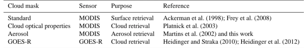
Table 1. The four cloud masks mentioned in this study. Only the MODIS aerosol and GOES-R cloud masks undergo analysis.
Cloud mask Sensor Purpose Reference
Standard MODIS Surface retrieval Ackerman et al. (1998); Frey et al. (2008) Cloud optical properties MODIS Cloud retrieval Platnick et al. (2003)
Aerosol MODIS Aerosol retrieval Martins et al. (2002) and this work
GOES-R GOES-R Cloud retrieval Heidinger and Straka (2010); Heidinger et al. (2012)
explicit masking of bright surfaces other than what is acci-dentally included in the MODIS aerosol cloud mask.
The Level 1-B reflectances are read in at 0.5×0.5 km res-olution, and the MODIS aerosol cloud mask is calculated at this resolution. We create coarser resolution masks by de-grading the resolution of this original mask. If a 0.5×0.5 km pixel is designated “cloudy” by the original mask, then all coarser masks that include that pixel are designated as “cloudy” as well. It takes only one single 0.5×0.5 km pixel to be cloudy to designate an entire degraded coarse resolu-tion pixel to be cloudy. In this way we are assuming a per-fect cloud mask that never makes mistakes as resolution be-comes coarser, or as the view angle bebe-comes more oblique. For this exercise we define the aerosol product retrieval box to be 8×8 km instead of the MODIS operational algorithm box size of 10×10 km. This makes degradation to coarser resolution easier.
In the MODIS operational algorithm, the retrieval pro-ceeds whenever there are at least 10 pixels remaining over ocean or 12 remaining over land after all de-selection
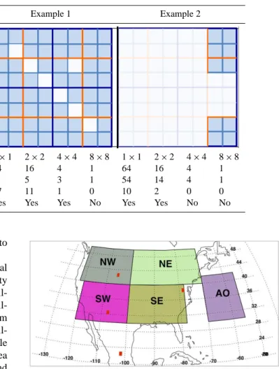
Table 2. Examples of different cloud configurations affecting retrieval opportunities in an 8×8 km product box. The last line denotes whether or not an aerosol retrieval would be made for the 8 km retrieval box, given the requirement that at least 10 % of the pixels are “cloud-free”.
Example 1 Example 2
Cloudy pixels (white) within a 8 km product box
els in box
1x1 2x2 4x4 8x8 1x1 2x2 4x4 8x8
in 64 16 4 1 64 16 4 1
7 5 3 1 54 14 4 1
els 57 11 1 0 10 2 0 0 Yes Yes Yes No Yes Yes No No
Pixel size (km) 1×1 2×2 4×4 8×8 1×1 2×2 4×4 8×8
Total pixels in 8 km box 64 16 4 1 64 16 4 1
# cloudy pixels 7 5 3 1 54 14 4 1
# clear pixels 57 11 1 0 10 2 0 0
8 km product Yes Yes Yes No Yes Yes No No
as finding appropriate surface reflectance, etc., will have to be considered as well.
Therefore, using actual MODIS observations of real scenes to form the cloud mask, we will ask how availability of aerosol retrieval varies as a function of pixel size. Avail-ability is defined as the number of 8 km product boxes avail-able for aerosol retrieval divided by the total number of 8 km boxes in the region or time period of interest. 100 % availabil-ity is the situation when every box in the domain is available to report an aerosol retrieval. In this study, our general area of interest is the Northern Hemisphere of the Americas and adjoining oceans, as shown in Fig. 5. We have also defined five large subdomains including four quadrants of continen-tal United States and a large region of midlatitude Atlantic Ocean (AO). The full domain, as designated in Fig. 5, en-compasses a larger area than the sum of the five subdomains, and therefore cannot be expected to represent the mean or median of the individual subdomains.
In the following analysis, level 1-B MODIS reflectances for the first week of every month from March 2009 through February 2010 are analyzed to provide a representative sam-ple of annual conditions. Seasonal statistics are calculated from three weeks of data, the first weeks of each of the three months that define each of the four seasons.
5.2 Regional and seasonal availability
The calculated availability using the data and methodology described in Sect. 5.1 is displayed in Fig. 6 for the full do-main and each regional subdodo-main as a function of instru-ment pixel size for each season. In every case, the coarser the resolution the fewer the number of 8 km boxes available for an aerosol retrieval. For example, in summer, at a spatial res-olution of 0.5×0.5 km, availability ranges between 40 % and
Fig. 5. The full study domain extends from the equator to 55◦N and from−139◦to−13◦W longitude. The full domain is divided into 5 subdomains: NW, NE, SW, SE and AO. The small red squares de-note specific locations at 1◦×1◦of more intense analysis: Wyoming (WY) in NW, New Mexico (NM) in SW, Virginia (VA) in SE, and Mexico (ME) south of SW.
65 %. This decreases to 33–58 % by degrading to 1×1 km pixel resolution. At a 4×4 km pixel resolution, availability has decreased further to 16–20 %. The rectangularly shaped 1×4 km pixels, with pixel areas of 4 km2, provide slightly less availability than do the 2×2 km pixels with the same pixel area. These are shown in Fig. 6 slightly offset from the 2 km pixel size at 2.25 km, only for plotting purposes.
Fig. 6. Calculated availability of an aerosol retrieval as a function of instrument pixel size for the full domain and subdomains defined in Fig. 5, for the four seasons.
snow pixels have to be eliminated from the retrieval also. Here, this factor may be contributing to the very low avail-ability numbers of the northern tier subdomains in winter.
Regionally, the southwest subdomain (SW) offers the highest availability of any of the domains at 0.5 km pixel resolution, but does not necessarily provide the highest avail-ability as spatial resolution degrades. For example, in Fall, by 8 km spatial resolution the SE and NE domains offer higher availability than does the SW. Differences in cloud type and morphology from region to region explain how this happens. Clouds in the SW tend to be small but widespread. At fine resolution, most product boxes are sparsely populated by clouds and retrievals are possible. However, as resolution de-grades almost every 8 km pixel contains a small cloud and is therefore designated cloudy. Availability drops. In contrast, clouds in the SE and NE are larger but clustered. At fine res-olution more product boxes in the SE and NE are affected by the large clouds making retrievals less likely overall. How-ever, the clear regions are particularly cloud-free, so that as
resolution degrades availability drops less quickly than for the small, widespread clouds of the SW.
Table 3 lists all calculated availabilities for each domain, season and spatial resolution. The seasonal and regional anal-ysis shows that an instrument with 4 km resolution generally can make less than half of the retrievals that a 0.5 km resolu-tion instrument can make, over the course of a season.
5.3 Differences between nadir and oblique angles
Table 3. Calculated availabilities using MODIS aerosol cloud mask with MODIS input radiances for five spatial resolutions, four seasons, and six domains including the full domain described in Sect. 5.1. Also shown are cloud fractions based on 0.5×0.5 km resolution cloud mask for each domain and season.
0.5×0.5 km 1×1 km 2×2 km 1×4 km 4×4 km 8×8 km Cloud- fraction Winter (DJF)
Full 0.34 0.26 0.20 0.18 0.13 0.06 0.81
AO 0.19 0.11 0.07 0.06 0.04 0.01 0.93
NE 0.07 0.05 0.04 0.03 0.02 0.01 0.96
NW 0.10 0.07 0.05 0.04 0.02 0.01 0.95
SE 0.28 0.24 0.20 0.19 0.14 0.05 0.81
SW 0.38 0.31 0.23 0.20 0.12 0.04 0.78
Spring (MAM)
Full 0.38 0.30 0.23 0.21 0.15 0.07 0.79
AO 0.44 0.36 0.31 0.29 0.24 0.16 0.72
NE 0.28 0.23 0.18 0.17 0.11 0.04 0.83
NW 0.25 0.19 0.13 0.12 0.07 0.02 0.88
SE 0.55 0.49 0.41 0.39 0.28 0.11 0.61
SW 0.60 0.51 0.39 0.36 0.23 0.07 0.63
Summer (JJA)
Full 0.43 0.34 0.26 0.24 0.17 0.07 0.76
AO 0.50 0.40 0.32 0.29 0.21 0.10 0.72
NE 0.40 0.31 0.24 0.22 0.16 0.07 0.77
NW 0.53 0.44 0.35 0.32 0.21 0.06 0.69
SE 0.51 0.40 0.32 0.30 0.21 0.07 0.70
SW 0.65 0.54 0.40 0.36 0.21 0.06 0.63
Fall (SON)
Full 0.43 0.33 0.26 0.24 0.17 0.07 0.76
AO 0.39 0.30 0.24 0.21 0.16 0.08 0.79
NE 0.43 0.38 0.33 0.32 0.25 0.13 0.69
NW 0.53 0.45 0.36 0.32 0.21 0.06 0.67
SE 0.60 0.54 0.48 0.46 0.36 0.17 0.55
SW 0.72 0.61 0.46 0.42 0.26 0.08 0.57
Numbers are fractions. AO = Atlantic Ocean, NE = Northeast, NW = Northwest, SE = Southeast, SW = Southwest.
edge. In this analysis, we also ignored the degradation, so that the nominal 8×8 km resolution pixel defined at nadir is actually 32×32 km at swath edge. All values of availability and cloud fraction presented in Fig. 6 and Table 3 are mix-tures of nadir and oblique angles, defined by pixel resolution at nadir, but consisting of an actual range of pixel sizes span-ning nadir values to 4 times nadir values.
To investigate the effect of pixel resolution degradation across the MODIS swath on aerosol retrieval availability, we divided the data into nadir views where sensor view angle is within 20◦of nadir, and oblique views where sensor view an-gle is greater than 50◦. Note that the full MODIS swath spans view angles±65◦. The results of this exercise are presented in Fig. 7 and Table 4 for the spring season.
The general trends identified using all view angles are the same when sorting into nadir and oblique angles. Both view angle subsets decrease availability as nominal pixel resolu-tion degrades, and the rates of decrease (the slopes in Fig. 7) are similar within each subdomain. The northern tier subdo-mains have the lowest availabilities, and the SW subdomain
has the highest availability, but it decreases more sharply as nominal pixel resolution is degraded.
Fig. 7. Calculated availability of aerosol retrieval as a function of instrument pixel size for the full domain and subdomains defined in Fig. 5, for the spring season, and separated into oblique angles with sensor view angle greater than 50◦(solid lines) and nadir angles with sensor view less than 20◦(dashed lines). The six domains analyzed are presented in two panels for visual clarity.
Table 4. Seasonal mean aerosol retrieval availabilities and cloud fraction for the full domain and subdomains during spring (MAM), divided into nadir views (sensor view angle<20◦)and oblique views (sensor view angle>50◦). Cloud fraction is for the native nominal resolution of MODIS, 0.5×0.5 km at nadir.
0.5×0.5 km 1×1 km 2×2 km 4×4 km 8×8 km Cloud- fraction nadir
Full 0.42 0.33 0.26 0.17 0.08 0.76
AO 0.42 0.34 0.29 0.22 0.15 0.74
NE 0.33 0.27 0.22 0.13 0.05 0.80
NW 0.30 0.24 0.18 0.10 0.02 0.84
SE 0.56 0.51 0.44 0.31 0.11 0.59
SW 0.65 0.57 0.46 0.27 0.08 0.58
oblique
Full 0.38 0.30 0.23 0.15 0.07 0.75
AO 0.47 0.40 0.35 0.29 0.21 0.67
NE 0.32 0.26 0.21 0.13 0.05 0.81
NW 0.18 0.12 0.08 0.03 0.01 0.93
SE 0.55 0.49 0.41 0.27 0.11 0.62
SW 0.53 0.43 0.31 0.17 0.05 0.71
5.4 Regional availability on a single day
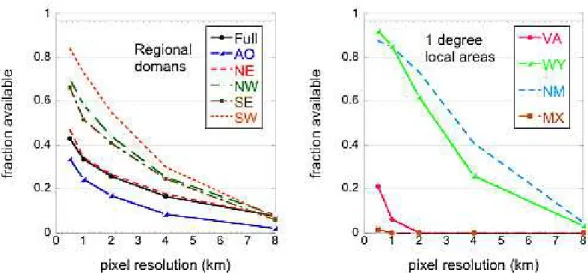
Not all applications will be satisfied in obtaining aerosol statistics on a seasonal basis only. Some applications will re-quire aerosol retrievals to be available within the region on a single day. Air quality forecasting and aerosol assimilation are such examples. To explore the availability in the five sub-domains and the full domain of Fig. 5, we calculate the avail-ability for a randomly selected day, 12 August 2010. The left panel of Fig. 8 shows the results.
There is greater spread of results from subdomain to sub-domain for one day in August, as compared with the summer panel of Fig. 6. Other differences include the low availability for the Atlantic Ocean domain for the one day, as compared
Fig. 8. (left) Aerosol retrieval availability for 12 August 2010 for the full domain and five subdomains defined by Fig. 5, and (right) for the four 1-degree squares representing local areas, as defined in Fig. 9.
from 0.5 km to 4 km causes a greater loss in the possible retrievals in almost every subdomain on that particular day than was evident in the seasonal analysis. In some cases, like the ocean, this leaves very few opportunities for retrieval. In other domains, the availability at 4 km remains above 25 %. However, at 8 km resolution, almost all domains are reduced to 10 % of their potential retrievals on this day.
5.5 Local availability on a single day
Calculations of aerosol retrieval availability over broad do-mains may be insufficient for applications that focus on a particular local area. For example, local air quality moni-toring and field experiment support require information on a much smaller scale than addressed above. To investigate local availability on a single day we again choose 12 August 2010 as a random day of interest and focus on four local re-gions indicated by the red dots in Fig. 5. Each dot represents a 1-degree square chosen for a variety of cloud conditions on this particular day. The four regions are shown using Terra-MODIS imagery in Fig. 9.
The availability was calculated for these local 1-degree squares on 12 August 2010 using the MODIS Level 1-B data much the same as was done for the larger domains. The right panel of Fig. 8 shows the results and Table 5 gives the results numerically. The very cloudy local areas of Virginia (VA) and Mexico (MX) barely offer any opportunity for retrieval. However, it is surprising that at 0.5 km the availability at VA is still 21 %. This opportunity for retrieval is closely tied to the 0.5 km resolution and essentially disappears even at 1 km. The Wyoming (WY) and New Mexico (NM) local areas are seen with a minimal amount of scattered small clouds. This situation permits over 80 % availability at 0.5 km and 1 km resolution. However, even though many clouds are not vis-ible in the images, there are sufficient randomly distributed
Fig. 9. Terra MODIS true color imagery of four local areas on 12 August 2010. The red box in each image represents a 1-degree square used to define a local region in the analysis. The four re-gions are Virginia (VA), Wyoming (WY), New Mexico (NM) and Mexico (MX).
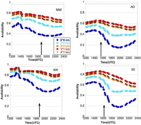
Fig. 10. Diurnal patterns of aerosol retrieval availability on 12 August 2010 for four different spatial resolutions for four subdomains, Northwest (NW), Atlantic Ocean (AO), Southwest (SW) and Southeast (SE), defined in Fig. 5. The availability was calculated using the GOES-R cloud mask applied to one day of GOES radiances archived at 5-min temporal resolution. The black arrows indicate time of Terra overpass. The 4×1 km is denoted by small brown circles that are almost exactly overlaid onto the 2×2 km orange curve.
6 Aerosol product availability from a geosynchronous satellite
A polar orbiting satellite such as Terra or Aqua passes over each location on Earth only once per day during daylight hours, except at high latitude. This permits MODIS gener-ally only one chance to retrieve aerosol at a particular loca-tion, per satellite, per day. A geosynchronous satellite, like GOES or the proposed Geostationary Coastal and Air Pol-lution Events (GEO-CAPE) mission, can observe each loca-tion every 5 min, although, operaloca-tionally, data collecloca-tion fre-quency is every 15 min. This temporal resolution can provide information on day time variation of aerosols when the sit-uation is mostly cloud-free. Previous studies have explored the diurnal aerosol signal (Smirnov et al., 2002; Zhang et al., 2012) and have even shown that statistics calculated at polar orbiting times reflect the statistics calculated from the full diurnal cycle (Kaufman et al., 2000), but none of these studies accounted for clouds interfering with the ability of a satellite to make a retrieval.
Even if a situation is too cloudy for an aerosol retrieval at the time of a polar orbiter’s overpass, perhaps opportu-nity will open at other times during the day and the geosyn-chronous instrument will be able to retrieve. Thus, it may be able to trade high temporal frequency over a region for high spatial resolution and increase the availability by making at least one retrieval on a single day within the domain of mea-surement.
Table 5. Calculated availabilities using MODIS aerosol cloud mask for 12 August 2010 for six spatial resolutions and ten domains including the four local areas shown in Fig. 8. Also shown are cloud fractions based on 0.5×0.5 km resolution cloud mask for each domain for this day.
0.5×0.5 km 1×1 km 2×2 km 1×4 km 4×4 km 8×8 km Cloud-fraction
Full 0.43 0.34 0.26 0.24 0.17 0.08 0.76
AO 0.34 0.25 0.17 0.14 0.09 0.02 0.86
NE 0.47 0.34 0.27 0.25 0.18 0.08 0.76
NW 0.70 0.58 0.44 0.39 0.25 0.08 0.60
SE 0.66 0.52 0.41 0.38 0.25 0.06 0.63
SW 0.84 0.73 0.55 0.50 0.30 0.07 0.49
VA 0.21 0.06 0 0 0 0 0.97
WY 0.92 0.85 0.62 0.53 0.26 0.03 0.51
NM 0.88 0.85 0.73 0.65 0.41 0.05 0.36
MX 0.02 0 0 0 0 0 1.00
scheme, as illustrated in Fig. 1 and similar to the lower left panel of Fig. 2.
Unfortunately, only one day of data is available. GOES data are generally archived at coarser temporal resolution (15 min), making this specific day of data unique. Because there is only one day of data, it is difficult to place the re-sults of the GOES analysis on the same par as the seasonal analysis applied to the MODIS data. Still, the GOES analy-sis provides a glimpse into what might be expected from a geosynchronous satellite in terms of aerosol retrieval avail-ability and the differences in availavail-ability between a cloud mask designed for an aerosol retrieval (MODIS) and one de-signed for cloud retrievals (GOES-R).
Availability was calculated in a similar procedure to what was described above for the MODIS aerosol cloud mask, but this time the GOES-R cloud product was used instead. As be-fore, availability is not the same as the “cloud-free” fraction. The input radiances are organized into 8 km retrieval boxes, and the number of “cloud-free” pixels are calculated within each box. A retrieval box is designated as “available for po-tential aerosol retrieval” if the number of cloud-free pixels exceeds 10 % of the total number of pixels in the retrieval box, the same as the threshold used with MODIS. Availabil-ity for the region and time period of interest is the number of retrieval squares available for retrieval divided by the to-tal number of 8 km retrieval squares. In the geosynchronous analysis, the finest spatial resolution is 1×1 km, which in turn is degraded to 1×4, 2×2, 4×4 and 8×8 km pixel sizes.
Figure 10 shows the diurnal patterns of availability for four of the five subdomains defined in Fig. 5 for the one day of analysis using the GOES-R cloud identification data set. The NE subdomain is not shown because it mimics the diurnal pattern of the AO subdomain. In all subdomains the diurnal pattern offers the greatest aerosol retrieval availability in the morning and the least in the afternoon. The coarser the pixel spatial resolution, the less the availability and the greater the amplitude of the diurnal availability signal. This is consis-tent with the growth of boundary layer clouds and general
increase of cloudiness expected in the afternoon over land. However, the AO subdomain also shows a strong decrease of availability in the afternoon at 4 km and especially 8 km pixel resolution. In the western subdomains we see a kink in the availability at 13:00 UTC at all spatial resolutions. In the west, it is still dark at 12:00 UTC (05:00 to 06:00 a.m.) over much of these subdomains. The kink is an artifact in the GOES-R cloud identification routine as it transitions from an all-infrared (IR) algorithm at night to a combined visible and IR algorithm during the day.
The overall availability is higher using the GOES-R data set than using the MODIS aerosol cloud mask, but some of the trends are similar. For example, the SW offers the highest availability on this day, while the AO offers the lowest. How-ever, during the morning hours the loss of retrieval availabil-ity with degradation of spatial resolution is not as severe as seen in Fig. 8, but increases severely in the afternoon. Still, the GOES-R cloud identifier permits at least 20 % availabil-ity at 8 km over all subdomains, while the MODIS aerosol cloud mask allows only less than 10 % at the same pixel res-olution for that day.
Fig. 11. Diurnal patterns of aerosol retrieval availability on 12 August 2010 for four different spatial resolutions for the four 1-degree local areas defined in Fig. 9. The availability was calculated using the GOES-R cloud mask applied to one day of GOES radiances archived at 5-min temporal resolution. Black arrows point to times of Terra overpass. The 4×1 km is denoted by small brown circles that are almost exactly overlaid onto the 2×2 km orange curve.
achieving diurnal aerosol consistency in situations of diurnal cloud variability lies outside the scope of this study.
The GOES-R cloud identification produces a wide range of availability as a function of spatial resolution. With in-creasing of cloudiness, there is a large difference in availabil-ity between 1–2 km pixel size and 4–8 km. In VA and MX, the two very cloudy regions, there are times during the late morning when the 1 km resolution produces almost 100 % availability simultaneous to the 8 km resolution producing 0 % availability. This contrasts with the MODIS aerosol cloud mask results of Fig. 8. Even at Terra overpass times of 16:45 UTC and 16:50 UTC when the MODIS aerosol cloud mask produced 10 % and 0 % availability at 1 km for VA and MX, respectively, the GOES-R cloud identifier produced nearly 100 % availability at 1 km. Figure 12 further demon-strates these differences for all domains and areas. In this figure the 12 August 2012 availabilities calculated from the MODIS and GOES-R cloud masks are plotted on the same plot for two different resolutions. The GOES-R availabilities shown in Fig. 12 correspond to time of Terra overpass for the
respective location (15:05 UTC for AO; 16:45 UTC for NE, SE and VA; 16:50 UTC for MX; 18:25 UTC for NW, SW, WY and NM). The GOES-R cloud identifier always allows for greater availability than the MODIS aerosol cloud mask for all domains and local areas. In some situations, especially the relatively cloud free local areas, the two cloud products result in similar levels of availability, but the difference be-tween the two increases as the cloudiness of the domain in-creases. This is because the two cloud products were devel-oped for different purposes, which will be discussed below.
7 Discussion and conclusions
Fig. 12. Aerosol retrieval availability for the full domain and the five subdomains defined in Fig. 5, as well as for the four local 1-degree areas defined in Fig. 9 for one day, 12 August 2010. Shown are the results from using the GOES-R cloud identifier applied to GOES data and the MODIS aerosol cloud mask applied to MODIS data, for 1 km resolution (left) and 4 km resolution (right). The GOES-R availabilities are calculated for the same time as MODIS overpass and are not diurnal averages.
we define it, is not the same as cloud free fraction, because aerosol retrievals are made after selecting ideal pixels for re-trieval within a larger box.
The cloud mask used for MODIS aerosol retrieval is de-signed to protect the aerosol product from cloud contamina-tion, even if the masking creates false positives for clouds. We see these false positives in the analysis when snowy re-gions and ocean glint contribute to the cloud fraction in the MODIS aerosol cloud mask. Another cloud mask, developed for GOES-R and applied to one day of GOES data (Heidinger and Straka, 2010), takes a different approach that attempts to minimize false positives. These different approaches create striking differences in aerosol retrieval availability for one day in the summer of 2010. In some situations the MODIS aerosol cloud mask resulted in essentially 0 % availability, while the GOES-R cloud mask that avoids false positives for clouds found 80 % availability. Clearly, a “one-size” cloud mask cannot fit all. Imposing a cloud mask developed to identify clouds will cause the aerosol retrieval to fail.
Because of these striking differences between availability calculated from the two cloud masks for collocated scenes, we conclude that the GOES-R availabilities calculated here are overly optimistic for aerosol retrievals. This conclusion is based on three reasons: (1) the MODIS aerosol cloud mask was developed specifically for application with an aerosol retrieval, while the GOES-R cloud mask was not; (2) the MODIS aerosol cloud mask is well-established in an aerosol context and has undergone a decade of evaluation, while this is the first time the GOES-R cloud mask was used in an aerosol context; (3) visually, the conditions seen in Fig. 9 for VA and MX contradict the 80 % to 90 % aerosol retrieval availability calculated using the GOES-R cloud mask, while the MODIS values of 0 to 10 % are more appropriate for these very cloudy scenes. The GOES-R cloud mask can be
used to learn about diurnal patterns, but should not be used for absolute availability.
The unanswered question from this analysis is what are the quantitative effects on the aerosol product using each of the cloud masks: the Ackerman et al. (1998) and Platnick et al. (2003) cloud masks from Table 1, as well as the MODIS aerosol cloud mask (Martins et al., 2002) and the GOES-R cloud mask (Heidinger and Straka, 2010). In this study we limit our analysis to product availability as a function of pixel size and do not address cloud contamination in the products. A thorough investigation of the effects of different cloud masks on aerosol retrievals is recommended for the fu-ture.
The results using MODIS show a decrease of availabil-ity as the sensor pixel size is made coarser. An instrument with a nominal 4 km footprint will lose 60 % to 70 % of the retrievals that it would have made with a nominal 0.5 km pixel instrument. An instrument with a nominal 8 km foot-print will lose 70 % to 85 % of its aerosol retrievals. We note that this study only considers clouds as it calculates avail-ability. There are many other situations besides cloudiness that will prevent an aerosol retrieval, most likely inappropri-ate surface reflectances such as sun glint, snow, ice, inland water, bright deserts, etc. Kahn et al. (2009) note that actual MODIS availability is close to 15 % on a global basis. That is at nominal 0.5 km resolution. While there is no guarantee that the availability calculated here for North America will trans-late directly to global conditions, if it does, then globally, a MODIS-like sensor and algorithm with 8 km pixel size will retrieve aerosol only over 3 % to 5 % of the Earth.
much as 40 %, meaning that there are 40 % less opportunities to make a retrieval at swath edge than at nadir. However, that drastic change was seen in only one subdomain. In other do-mains the differences in availability between nadir and swath edge were within 10–20 %. Over land, the tendency is for oblique angles to be cloudier because the sensor is seeing cloud sides as well as cloud tops. However, over ocean, the nadir views are affected by sun glint, causing artificial en-hancement of cloud cover at nadir which overwhelms the in-creased cloudiness of the oblique views. Over ocean, aerosol product availability is higher at swath edge than at nadir.
The analysis of the GOES-R cloud mask applied to geosta-tionary satellite radiances from GOES reveals interesting di-urnal patterns, but because this analysis is applied to only one day, it is difficult to make firm conclusions. The one day anal-ysis suggests the possibility that regions overcast with clouds at typical polar orbiting satellite overpass times may open up to aerosol retrievals either early or late in the day. The diurnal availability pattern is most significant at the coarser spatial resolutions, suggesting that an aerosol retrieval using 8 km radiance may be almost as available in the early morn-ing as the 1 km retrieval is at midday. This diurnal pattern has some regional and seasonal variation. However, from a scientific perspective the early morning aerosol that can be retrieved may have very different properties than the aerosol that cannot be retrieved. We note that based on this analy-sis there is little possibility of resolving the diurnal cycle of aerosol properties from satellite if using an instrument with a 4 km or 8 km footprint. The availability at midday is too low. However, the diurnal analysis was limited to just one day, and may not be representative of other conditions.
New satellite sensors are being discussed with a variety of possible spatial resolutions. GEO-CAPE is a proposed geo-stationary mission with part of its objectives to character-ize and monitor air pollution, including aerosols. The results here suggest that at 1 or 2 km resolution, GEO-CAPE will have sufficient aerosol product availability even on a day-to-day basis for a local area. The difference between 1×1, 2×2 and 1×4 km is not significant. However, by 4×4 km, the scarcity of aerosol retrievals will begin to hamper applica-tions. Another potential satellite sensor for aerosol retrievals is the Aerosol Polarimeter Sensor (APS) that was launched as part of the Glory mission, but did not reach orbit. A re-flight is possible. With its 6 km footprint at nadir and 20 km at far viewing angles, clouds will almost always be in APS’s field of view. The results here reinforce the understanding that cloud mitigation efforts need to be developed for APS, using its polarization capability, or substantial aerosol prod-uct availability will be lost.
Acknowledgements. The authors thank the two anonymous referees
who each provided extensive comments on the discussion paper. Answering their questions improved the final paper immensely. The authors would also like to thank the GEO-CAPE aerosol workinggroup for their helpful discussion during the genesis of
this work. The work was supported by NASA as part of efforts for GEO-CAPE aerosol science definition under the direction of Jay Al-Saadi.
Edited by: O. Dubovik
References
Ackerman, S. A., Strabala, K. I., Menzel, W. P., Frey, R. A., Moeller, C. C., and Gumley, L. E.: Discriminating clear-sky from clouds with MODIS, J. Geophys. Res., 103, 32141–32157, 1998. Ackerman, S. A., Frey, R., Strabala, K., Liu, Y., Gumley, L.,
Baum, B., and Menzel, P.: Discriminating clear-sky from clouds with MODIS. Algorithm Theoretical Basis Document (MOD35), available at: http://modis-atmos.gsfc.nasa.gov/ docs/ MOD35 ATBD Collection6.pdf, version 6.1, October 2010. Al-Saadi, J., Szykman, J., Pierce, R. B., Kittaka, C., Neil, D., Chu,
D. A., Remer, L., Gumley, L., Prins, E., Weinstock, L., MacDon-ald, C., Wayland, R., Dimmick, F., and Fishman, J.: Improving national air quality forecasts with satellite aerosol observations, B. Am. Meteorol. Soc., 86, 1249–1264, doi:10.1175/BAMS-86-9-1249, 2005.
Charlson, R. J., Ackerman, A. S., Bender, F. A.-M., Anderson, T. L., and Liu, Z.: On the climate forcing consequences of the albedo continuum between cloudy and clear air, Tellus B, 59, 715–727, doi:10.1111/j.1600-0889.2007.00297.x, 2007.
Chu, D. A., Kaufman, Y. J., Zibordi, G., Chern, J. D., Mao, J., Li, C., and Holben, B. N.: Global monitoring of air pollution over land from EOS-Terra MODIS, J. Geophys. Res., 108, 4661, doi:10.1029/2002JD003179, 2003.
EPA (United States Environmental Protection Agency): The plain English guide to the national Clean Air Act, Office of Air Quality Planning and Standards, Research Triangle Park NC, EPA-456/K-07-001, available at: http://www.epa.gov/airquality/ peg caa/pdfs/peg.pdf, 2007.
Frey, R. A., Ackerman, S. A., Liu, Y. H., Strabala, K. I., Zhang, H., Key, J. R., and Wang, X. G.: Cloud detection with MODIS. Part I: Improvements in the MODIS cloud mask for collection 5, J. Atmos. Ocean. Tech., 25, 1057–1072, 2008.
Gao, B. C., Kaufman, Y. J., Tanre, D., and Li, R.-R.: Dis-tinguishing tropospheric aerosols from thin cirrus clouds for improved aerosol retrievals using the ratio of 1.38-µm and 1.24-1.38-µm channels, Geophys. Res. Lett., 29, 1890, doi:10.1029/2002GL015475, 2002.
Gupta, P. and Christopher, S. A.: Particulate matter air quality assessment using integrated surface, satellite, and meteorolog-ical products: Multiple regression approach, J. Geophys. Res.-Atmos., 114, D14205, doi:10.1029/2008JD011496, 2009. Heidinger A. and Straka III, W. C.: GOES-R ABI Cloud Mask
The-oretical Basis Document, version 2.0, GOES-R Program Office, 2010.
Heidinger, A. K., Evan, A. T., Foster M. J., and Walther, A.: A Naive Bayesian Cloud Detection Scheme Derived from CALIPSO and Applied to PATMOS-x, J. Appl. Meteor. Climatol., 51, 1129– 1144. doi:10.1175/JAMC-D-11-02.1, 2012.
Jethva, H. and Torres, O.: Satellite-based evidence of wavelength-dependent aerosol absorption in biomass burning smoke inferred from Ozone Monitoring Instrument, Atmos. Chem. Phys., 11, 10541–10551, doi:10.5194/acp-11-10541-2011, 2011.
Kahn, R. A., Nelson, D. L., Garay, M., Levy, R. C., Bull, M. A., Martonchik, J. V., Diner, D. J., Paradise, S. R., Wu, D. L., Hansen, E. G., and Remer, L. A.: MISR Aerosol product attributes, and statistical comparisons with MODIS, IEEE T. Geosci. Remote, 12, 4095–4114, 2009.
Kahn, R. A., Gaitley, B. J., Garay, M. J., Diner, D. J., Eck, T., Smirnov, A., and Holben, B. N.: Multiangle Imaging SpectroRa-diometer global aerosol product assessment by comparison with the Aerosol Robotic Network, J. Geophys. Res., 115, D23209, doi:10.1029/2010JD014601, 2010.
Kaufman, Y. J., Holben, B. N., Tanr´e, D., Slutsker, I., Smirnov, A., and Eck, T. F.: Will aerosol measurements from Terra and Aqua polar orbiting satellites represent aerosol abun-dance and properties?, Geophys. Res. Lett., 27, 3861–3864, doi:10.1029/2000GL011968, 2000.
Kaufman, Y. J., Tanre, D., and Boucher, O.: A satellite view of aerosols in the climate system, Rev. Nature, 419, 215–223, 2002. Koren, I., Remer, L. A., Kaufman,Y. J, Rudich, Y., and Martins, J. V.: On the twilight zone between clouds and aerosols, Geophys. Res. Lett., 34, L08805, doi:10.1029/2007GL029253, 2007. Krewski, D., Burnett, R. T., Goldberg, M. S., Hoover, K.,
Siemi-atycki, J., Jerrett, M., Abrahamowicz, A., and White, W. H.: Re-analysis of the Harvard six cities study and the American Cancer Society study of particulate air pollution and mortality, A special report of the institute’s particle epidemiology reanalysis project, 97 pp., Health Effects Inst., Cambridge, Mass, 2000.
Marshak, A., Wen, G., Coakley, J., Remer, L., Loeb, N. G., and Cahalan, R. F.: A simple model for the cloud adjacency effect and the apparent bluing of aerosols near clouds, J. Geophys. Res., 113, D14S17, doi:10.1029/2007JD009196, 2008.
Martins, J. V., Tanr´e, D., Remer, L., Kaufman, Y., Mattoo, S., and Levy, R.:MODIS Cloud screening for remote sensing of aerosols over oceans using spatial variability, Geophys. Res. Lett., 29, 8009, doi:10.1029/2001GL013252, 2002.
Platnick, S., King, M. D., Ackerman, S. A., Menzel, W. P., Baum, B. A., Riedi, J. C., and Frey, R. A.: The MODIS cloud products: Al-gorithms and examples from Terra, IEEE, Trans. Geosci. Remote Sens., 41, 459–473, doi:10.1109/TGRS.2002.808301, 2003. Pope III, C. A., Burnett, R. T., Thun, M. J., Calle, E. E., Krewski,
D., Ito, K., and Thurston, G. D.: Lung cancer, cardiopulmonary mortality and long-term exposure to fine particulate air pollution, J. Amer. Med. Assoc., 287, 1132–1141, 2002.
Prados, A., Kondragunta, S., Ciren, P., and Knapp, K.: The GOES Aerosol/Smoke Product (GASP) over North America: Compar-isons to AERONET and MODIS Observations, J. Geophys. Res., 112, D15201, doi:10.1029/2006JD007968, 2007.
Remer, L. A., Kaufman, Y. J., Tanr´e, D., Mattoo, S., Chu, D. A., Martins, J. V., Li, R. R., Ichoku, C., Levy, R. C., Kleidman, R. G., Eck, T. F., Vermote, E., and Holben, B. N.: The MODIS aerosol algorithm, products and validation, J. Atmos. Sci., 62, 947–973, 2005.
Remer, L. A., Chin, M., DeCola, P., Feingold, G., Halthore, R., Kahn, R. A., Quinn, P. K., Rind, D., Schwartz, S. E., Streets, D., and Yu, H.: Executive Summary, Atmospheric Aerosol Prop-erties and Climate Impacts, in: A Report by the U.S.
Cli-mate Change Science Program and the Subcommittee on Global Change Research, edited by: Chin, M., Kahn, R. A., and Schwartz, S. E., National Aeronautics and Space Administration, Washington, DC, USA, 2009.
Samet, J. M., Dominici, M. D. F., Curriero, F. C., Coursac, I., and Zeger, S. L.: Fine particulate air pollution and mortality in 20 U.S. Cities, 1987–1994, New. Engl. J. Medicine, 343, 1742– 1749, doi:10.1056/NEJM200012143432401, 2000.
Smirnov, A., Holben, B. N., Eck, T. F., Slutsker, I., Chatenet, B., and Pinker, R. T.: Diurnal variability of aerosol optical depth ob-served at AERONET (Aerosol Robotic Network) sites, Geophys. Res. Lett., 29, 2115, doi:10.1029/2002GL016305, 2002. Stier, P., Feichter, J., Kinne, S., Kloster, S., Vignati, E., Wilson, J.,
Ganzeveld, L., Tegen, I., Werner, M., Balkanski, Y., Schulz, M., Boucher, O., Minikin, A., and Petzold, A.: The aerosol-climate model ECHAM5-HAM, Atmos. Chem. Phys., 5, 1125–1156, doi:10.5194/acp-5-1125-2005, 2005.
Tanr´e, D., Br´eon, F. M., Deuz´e, J. L., Dubovik, O., Ducos, F., Franc¸ois, P., Goloub, P., Herman, M., Lifermann, A., and Waquet, F.: Remote sensing of aerosols by using polarized, directional and spectral measurements within the A-Train: the PARASOL mission, Atmos. Meas. Tech., 4, 1383–1395, doi:10.5194/amt-4-1383-2011, 2011.
Torres, O., Tanskanen, A., Veihelman, B., Ahn, C., Braak, R., Bhar-tia, P. K., Veefkind, P., and Levelt, P.: Aerosols and Surface UV Products from OMI Observations: An Overview, J. Geophys. Res., 112, D24S47, doi:10.1029/2007JD008809, 2007. van Donkelaar, A., Martin, R. V., and Park, R. J.: Estimating
ground-level PM2.5using aerosol optical depth determined from
satellite remote sensing, J. Geophys. Res.-Atmos., 111, D21201, doi:10.1029/2005JD006996, 2006.
van Donkelaar, A., Martin, R. V, Levy, R. C., DaSilva, A. M., Krzyzanowski, M., Chubarova, N. E., Semutnikova, E., and Cohen, A. J.: Satellite-based estimates of ground-level fine particulate matter during extreme events: A case study of the Moscow fires in 2010, Atmos. Environ., 45, 6226–6232, doi:10.1016/j.atmosenv.2011.07.068, 2011.
Waquet, F., Ri´edi, J., Labonnote, L.-C., Goloub, P., Cairns, B., Deuz´e, J.-L., and Tanr´e, D.: Aerosol remote sensing over clouds using the A-Train observations, J. Atmos. Sci., 66, 2468–2480, doi:10.1175/2009JAS3026.1, 2009.
Waquet, F., Riedi, J., Labonnotte, L., Thieuleux, F., Ducos, F., Goloub, Ph., and Tanr´e, D.: Aerosols remote sensing over clouds using the A-train observations, A-Train Symposium, New Or-leans, USA, 25–28 October, 2010.
Wen, G. Y., Marshak, A., and Cahalan, R. F.: Impact of 3-D clouds on clear-sky reflectance and aerosol retrieval in a biomass burn-ing region of Brazil , IEEE, Geosci. Remote Sens. Lett., 3, 169– 172, doi:10.1109/LGRS.2005.861386, 2006.
Yu, H., Kaufman, Y. J., Chin, M., Feingold, G., Remer, L. A., An-derson, T. L., Balkanski, Y., Bellouin, N., Boucher, O., Christo-pher, S., DeCola, P., Kahn, R., Koch, D., Loeb, N., Reddy, M. S., Schulz, M., Takemura, T., and Zhou, M.: A review of measurement-based assessments of the aerosol direct ra-diative effect and forcing, Atmos. Chem. Phys., 6, 613–666, doi:10.5194/acp-6-613-2006, 2006.
doi:10.1029/2005GL023254, 2005.
Zhang, Y., Yu, H., Eck, T. F., Smirnov, A., Chin, M., Remer, L., Bian, H., Tan, Q., Levy, R., Holben, B. N., and Piazzolla, S.: