Series V: Economic Sciences • Vol. 9 (58) No. 1 - 2016
Does government spending boost
economic growth in Europe?
Florin Teodor BOLDEANU
1, R
ă
zvan IALOMI
Ţ
IANU
2Abstract: The article aims to analyse the evolution of budgetary expenditures and their relationship with economic growth, especially in the EU countries and three non-EU countries - Switzerland, Norway and Iceland during 1991 - 2012. To test the link between government spending and economic growth the research used the United Nation Classification of the Functions of Government and three econometrical regression methods – ordinary least square, least squares dummy variable and the generalized method of moments. Statistical results for the 10 categories of expenditure have shown that economic affairs, environmental protection, recreation, culture and religion and social protection have a significant impact on economic growth. Also the recent economic crisis and the EU accession influenced the variation of GDP/capita.
Key-words: economic growth, COFOG, economic crisis, public spending, panel data, GMM
1. Introduction
The study aims to analyse the evolution of budgetary expenditures and their relationship with economic growth, especially in the EU countries and three non-EU countries - Switzerland, Norway and Iceland during 1991 - 2012. For this endeavour the article uses the United Nation division of government spending (Classification of the Functions of Government) and three econometrical regression methods – ordinary least square, least squares dummy variable and the generalized method of moments.
Based on the developments of econometric theory proposed by Arellano and Bover (1995), Blundell and Bond (1998) and Wooldridge (2002), we propose a dynamic model estimated by using the GMM method.
Governments apply different strategies for sizing public spending depending on the national and international context. Thus, in times of economic crisis the state is forced to allocate funds for social and economic affairs necessary to support its
1
Lucian Blaga University of Sibiu, [email protected]
2
development. The degree of economic development has a significant impact on the structure and volume of public expenditure, as developing countries need a sustained increase of their public spending so as to minimize the gap between them and the developed ones.
In the economic research studies there are many conflicting views regarding the effects of public expenditure on economic growth. In addition to providing social protection and transfers to maintain an optimal level of social welfare, the government invests in the economy both in the public sector (infrastructure, allocation of budgetary resources) and in the private sector to so as to increase productivity.
Short-term unproductive expenditures in education and health can facilitate long-term growth of labour productivity. In addition, the government can provide information for the economic environment, reduce financial risks and change the incentives. But many economists believe that public goods provided by the state may be ineffective. Also there are negative effects on economic growth by amending tax that doesn’t stimulate economic development and by the somewhat inefficient transfer mechanism between ministries. Raising taxes can cause a misallocation of surplus funds and may also cause a constraint for private sector.
Based on the research of Laura Braşoveanu (2008), Holzner (2011),
Miyakoshi et al. (2010) and others, the paper continues their analysis using functional classification of government expenditures by sectors.
We selected a sample of 30 European countries, both developed countries and developing ones. Due to the economic crisis the European governments have chosen to reduce part of their public expenditure to counter the economic and financial contagion. In this paper we analysed whether public expenditure had a significant effect on economic growth.
The remainder of the article is divided as follows: Section 2 addresses the literature review. Section 3 presents the methodology and the data used for the research. Section 4 the results obtained and Finally, Section 5 contains concluding remarks.
2. Literature review
The recent empirical studies show that the structure of public spending is more important than the overall level of expenditure, providing a clearer picture for policy makers to intervene effectively in the economy and to achieve long-term growth.
implications were very important for modelling and understanding the effects of government intervention on economic growth
Robert Barro (1991) published a study for 98 developed and developing countries to capture the link between public investment and economic growth in the period 1965-1985. The relationship is positive but not statistically significant.
Using the existing information about the linkage between public spending and economic growth, Devarajan (1996) attempted to investigate how changing the structure of government investment would affect GDP. This article was considered one innovative for the time. Devarajan et al.'s (1996) study was based on a panel of 43 developing countries. The period they had chosen was 1970-1990. For independent variables they used defence spending, education, health, transport and communications as both current and capital investment.
Devarajan et al. (1996) are of the opinion that the influence of public spending depends not only on their nature - spending productive, unproductive - but also the size of the percentage of GDP. The authors concluded that the present growth of public current expenditure has a significant and positive influence on economic growth. Capital expenditures have a negative impact on GDP per capita, and therefore these expenses, even if they are productive, used in excess, can become unproductive for the economy. Their empirical results showed that developing countries wrongly allocated public investments relying more on capital expenditure to the detriment of current expenditure.
Also the Romanian research literature studied the complex mechanism
between public expenditure and economic growth. Iulian and Laura Braşoveanu
(2008) conducted an econometric test to capture the correlation between expenditure (% of GDP) and economic growth in Romania during 1990-2011.The classification used by the authors divides public spending in three categories: productive spending (which stimulates growth), unproductive expenditure (braking effect of economic development) and other expenses. Like in our present study, they used also the 10 categories listed in by the United Nations Classification of the Functions of Government, but the aggregated them in 3 major components.
Their paper is a theoretical foundation and a practical test of how public spending affects economic growth in Romania. At first glance, the dynamics of economic growth is negatively correlated with expenditure (% of GDP). The two authors believe that this is explainable due to a decreasing relationship between government size and the level of development in a country.
After applying statistical simulation the authors found that all the categories of expenditure adversely affect economic growth in Romania.
Bingxin Yu et al (2009) studied the impact of expenditure patterns on the change of GDP in 44 developing countries in Asia, Africa and Latin America in the period 1980 to 2004 (totalling 80% of the GDP of countries in that category). To determine the effects of public spending (agriculture, education, health, telecommunications, social security and defence) on growth, the authors used the generalized method of moments GMM. They found that there is a correlation between public spending and GDP growth, but each of the different categories of expenditure affects the dependent variable depending on the region. Thus, in Africa, the expenditure for development (human capital) had a positive effect on economic development. In Asia capital expenditures, agriculture and education have positive influence, while in Latin America it was found that no category of expenditure promotes economic growth.
The influence of public spending on growth was studied also using the GMM, by Arusha C. (2009), which took into account both the size of public expenditure components and a quality factor - political governance. The research reveals that the influence of public spending varies by country, as it appears that only in countries with very good governance the expenditures are used more efficiently, with a positive effect on the economy of the states. The results highlight the need for good governance along with increased public consumption which will result in a sustainable growth.
Lamartina and Zaghini (2008) and Arpaia and Turrini (2008) tested the link between public spending and economic growth using the Wagner's Law.
Results for the first authors confirms Wagner's theory, due to the use of the coefficient of elasticity of public spending relative to GDP, which takes values above par (at a 1% increase in GDP, general government expenditure increased by 1,028%). For the second article, the applied cointegration tests show that the degree of economic development and public expenditure are linked by a long-term stable relationship. The result shows that for less developed countries with a high aging population, less indebted, public spending grow faster than GDP per capita. The study also points out that on average, three years are required for the change of public expenditure to cancel their long-term deviation to potential GDP.
3. Methodology and data
To capture the influence of public spending on economic growth for the 30 countries analysed (EU 27 and Switzerland, Norway and Iceland) we chose a multiple linear regression model using panel data. Using GMM, OLS and LSDV methods we empirically estimated the effects public expenditures have on growth.
Public expenditure data were collected from the Eurostat database. Data on total public expenditure and GDP per capita were collected from the statistical AMECO-Eurostat database.
Many of the economic articles and research studies use panel data models to understand the links between the variables. For example, using panel data models to estimate demand and supply (current demand depends on the past one), the dynamic equations for the evolution of wages, unemployment, capital investment and other subjects.
We started with the following simple regression:
, (1)
where,
yit - ln (GDP / capita);
GE it is the vector of the 10 expenditures (% of GDP) (S - General public
services (% of GDP); D- Defence (% GDP); A - Public Order and Safety (% GDP),
AE - economic affairs (% GDP) M - environmental protection (% of GDP); L – Housing and community amenities (% of GDP); H - Health (% GDP); C - Culture, recreation and religion (% GDP) E - Education (% GDP) P - Social
protection (% of GDP))
Dit is a vector of dummy variables (Member State - Accession to the European
Union, Crisis - economic and financial crisis of 2008, Development - developed or emerging countries)
u it - two-component vector for statistical errors
Index i tracks the cross-sectional dimension of the dataset from 1 to 30 (thirty countries), while t is the time index running from 1991 to 2012.
(2)
where
µ i = individual fixed effects, by a normal distribution law ( )
ε it - error term, by a normal distribution law ( )
GDP in this period consisting of both boom and recession years, we opted for logarithms of the variable y.
The model contains the following dummy variables:
• Member States -we wanted to analyse whether the EU accession for the countries of the sample has an influence on economic growth. The variable takes the value 1 for the years when the state analysed is part of the European community, and 0 for the years when the state is not a part of the European Union;
• Crisis - reflects the emergence of the economic and financial crisis, so we want to observe its impact on economic growth. In the period 2008-2011, when the global economic and financial crisis took place the dummy variable takes the value 1 and 0 in other years;
• Development - reflects the status of development of the countries analysed, namely whether they are developed or developing countries. The World Bank and IMF published a report in 2012 listing the developing countries. The dummy variable takes the value 0 for the state included in the developing country category and 1 if they are not in this class.
According to the research work of the authors Bingxin Yu (2009) and Bond et al (2002), to correct the effects produce by the GMM model and to address unobserved heterogeneity as in models with fixed effects, we applied variable differentiation and rewrite the model as follows:
(3)
Before analysing the links between private and public expenditure and economic growth, we will check the following conditions:
a. If the data series of GDP / capita and public and private sectors are stationary
b. If the series are cointegrated I (1)
Zaghini and Lamartina (2008) used the Hadri, Levin-Lin-Chu, Breitung, Pesaran, Fisher test to check the two conditions above. The same tests were used by Arpaia and Turrini (2008) to check stationary and cointegration for GDP / capita and the independent variables for a panel of homogeneous data.
Since the panel data analysed in this work is not balanced we should perform additional statistical tests to check stationary and cointegration. We use the new econometrical program Stata v12 to get the results of the statistical tests.
3.1. Validating the model
The result obtained after applying the Hausman test is as follows:
Test: Ho: difference in coefficients not systematic chi2(13) = (b-B)'[(V_b-V_B)^(-1)](b-B)
= 51.75 Prob>chi2 = 0.0000 (V_b-V_B is not positive definite)
(Source: Stata v12)
Table 1. Hausman test results for panel data with dummy variables
Obtaining a probability lower than 5% (Prob> Chi2 = 0.0000), concludes that for the panel data it is best to use a fixed effect model.
To confirm or deny the presence of heteroscedasticity, we used the Wald test and got the following result:
Modified Wald test for Group Wise heteroscedasticity in fixed effect regression model
H0: sigma(i)^2 = sigma^2 for all i chi2 (30) = 12373.44 Prob>chi2 = 0.0000
(Source: Stata v12)
Table 2. Wald test results (heteroscedasticity) for panel data with dummy variables
Since the probability is less than 5% significance threshold (> 0.0000) the null hypothesis that states the presence of homoscedasticity phenomenon is rejected, so that the panel data reviewed affirms the presence of heteroscedasticity.
In general, the failure of the homoscedasticity hypothesis is base on two categories of factors: the wrong specification of the regression model or the nature of the phenomenon studied. In the presence of heteroscedasticity, standard errors of the estimators are misplaced and we should use robust errors to correct the phenomenon. The most likely deviation from homoscedastic errors in the context of panel data is due to specific individual variance. When errors are homoscedastic in cross-sectional units, but their variance is different between units we are dealing with heteroscedasticity between groups.
The serial correlation of the data will be tested using the model applied by Wooldridge (2002). He conducted a test of serial autocorrelation for panel data. We obtained the following results:
Wooldridge test for autocorrelation in panel data H0: no first-order autocorrelation
F (1, 29) = 230.101 Prob > F = 0.0000
(Source: Stata v12)
Table 3. Wooldridge test results (autocorrelation) for panel data with dummy variables
According to the results obtained, the H0 hypothesis is accepted. The panel data set containing correlated series. Serial correlation can produce inefficient estimates of standard errors or misinterpretations. The model does contain data auto correlated. Because of heteroscedasticity and serial correlation, we will use cluster-robust standard errors.
To check stationarity of the series we will use Fisher's test. The Hadri test, Levin-Lin-Chu, Breitung and Pesaran are also used to verify statonarity, but for an unbalanced panel the results obtained contain errors.
We will use the Fisher test at lag 0 and 1 to see the changes on the probability of rejecting the null hypothesis. According to the stationary results, all 11 variables analysed (the GDP / capita and the 10 categories of public expenditure) have rejected the null hypothesis. These series are stationary. To limit the paper we did not include these results, but they may be provided by the authors on request.
4. Results
To continue the analysis we will apply a simple regression method of least squares (OLS – ordinary least squares ), a model with fixed and dummy variables also using least squares (LSDV –least squares dummy variables) and generalized method of moments (GMM). These methods will provide relevant information to determine the link between economic growth and public expenditure for the 10 categories according to functional classification.
Using the Parm test we will determine if we should include a regression with fixed effects and dummy variables for the years analysed. The model contains three dummy variables and the test results are as follows:
F(22, 486) = 22.64 Prob > F = 0.0000
(Source: Stata v12)
The results show that the H0 hypothesis is rejected. All the coefficients of time dummy variables are equal to zero, because Prob> F = 0.0000, so less than the 10% threshold. Therefore, we conclude the fact that is necessary to use dummy variables.
We will use the first differential of the econometric model to analyse the link between public spending and growth for the panel data during 1991-2012. Due to the use of differential function the panel is reduced by 60 observations. The shape of the differential function is as follows:
(4)
We will analyse the OLS regression to determine the effects on growth of public expenditure. The results of the OLS model – ordinary least squares can be seen in the table below:
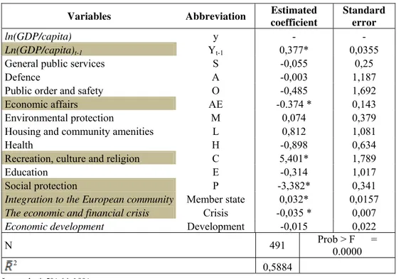
Variables Abbreviation Estimated
coefficient
Standard error
ln(GDP/capita) y - -
Ln(GDP/capita)t-1 Yt-1 0,377* 0,0355
General public services S -0,055 0,25
Defence A -0,003 1,187
Public order and safety O -0,485 1,692
Economic affairs AE -0.374 * 0,143
Environmental protection M 0,074 0,379
Housing and community amenities L 0,812 1,081
Health H -0,898 0,634
Recreation, culture and religion C 5,401* 1,789
Education E -0,314 1,017
Social protection P -3,382* 0,341
Integration to the European community Member state 0,032* 0,0157 The economic and financial crisis Crisis -0,035 * 0,007
Economic development Development -0,015 0,022
N 491 Prob > F =
0.0000 2
0,5884
Legend : * 5% ** 10%
(Source: Stata v12)
Table 5. Results for the OLS regression
The coefficient of determination denotes the percentage of the total variation of the dependent variable explained by the independent variables chosen. Thus, 58.84% of the variation of this ratio is explained by exogenous variables included in the model.
The Fisher test examines the hypothesis that all coefficients of the regression equation to be simultaneously zero. In Stata this hypothesis is rejected if Prob>F is very close to zero. In our case the probability is 0.00.
Prob> F shows the critical probability test, so if this value is less than 0.05 rejecting the hypothesis of lack of significance of the independent variables in favour of the hypothesis that the regression model is significant.
So we can reject the null hypothesis and conclude that at least a regression of the 13 is statistically significant. The model was well constructed.
Another aspect of the regression table refers to the value of "p" for each independent variable. This shows whether the variable has or does not have an effect on the dependent variable. 5% is the threshold. If the “p" value for a variable is less than this threshold, it means that the variable influences indeed the dependent variable. Also, it should be noted that, although in theory the threshold is considered to be 0.05 (5%), articles and papers consider all variables whose threshold is maximum 10%.
Because the threshold is relevant only for the following variables: ln (GDP /
capita)t-1, economic affairs, culture, recreation and religion, social protection, and
two dummy variable – Members state and economic crisis, we will retest the model using these variables and we will try to see what influences they have on economic growth. The other variables are not statistically significant to determine the variation of GDP / capita.
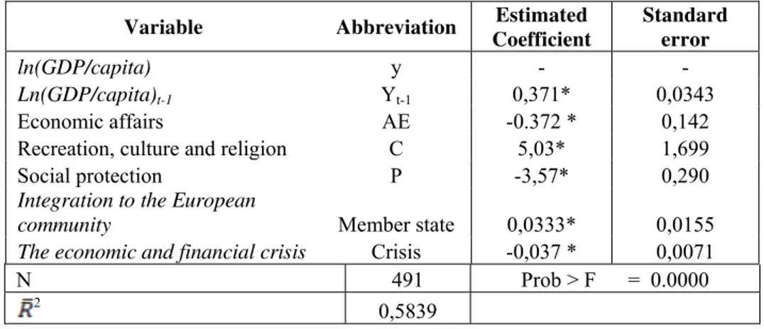
Variable Abbreviation Estimated
Coefficient
Standard error
ln(GDP/capita) y - -
Ln(GDP/capita)t-1 Yt-1 0,371* 0,0343
Economic affairs AE -0.372 * 0,142
Recreation, culture and religion C 5,03* 1,699
Social protection P -3,57* 0,290
Integration to the European
community Member state 0,0333* 0,0155
The economic and financial crisis Crisis -0,037 * 0,0071
N 491 Prob > F = 0.0000
2
0,5839
Legend : * 5% ** 10%
(Source: Stata v12)
There is a negative relationship between economic affairs and social protection and the economic growth. Thus, at 1 p.p. increase of economic affairs expenditure the GDP / capita decreases by 0.372 % and with negative 3.57% for increasing the social protection expenditure. Barro and Sala-i-Martin (1995) stated that these categories of government spending are unproductive for the economy. So our results are in line with their findings.
The expenditure for culture, recreation and religion are evolving in the same direction with the economic growth, so their growth increases by 1 percentage to obtain 5.03% increase in GDP / capita.
In terms of dummy variables, it can also be said that EU membership had a favourable effect on growth, but one not so considerably. But the economic crisis has had an adverse effect on GDP per capita.
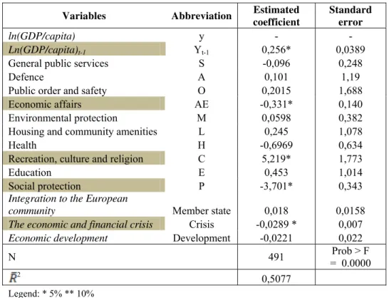
We will continue the analysis using LSDV- method of least squares mean model with dummy variables and fixed effects by country.
Variables Abbreviation Estimated
coefficient
Standard error
ln(GDP/capita) y - -
Ln(GDP/capita)t-1 Yt-1 0,256* 0,0389
General public services S -0,096 0,248
Defence A 0,101 1,19
Public order and safety O 0,2015 1,688
Economic affairs AE -0,331* 0,140
Environmental protection M 0,0598 0,382
Housing and community amenities L 0,245 1,078
Health H -0,6969 0,634
Recreation, culture and religion C 5,219* 1,773
Education E 0,453 1,014
Social protection P -3,701* 0,343
Integration to the European
community Member state 0,018 0,0158
The economic and financial crisis Crisis -0,0289 * 0,007
Economic development Development -0,0221 0,022
N 491 Prob > F
= 0.0000 2
0,5077
Legend: * 5% ** 10%
(Source: Stata v12)
Table 7. Results for the LSDV regression
financial crisis explain the variation of GDP/capita in proportion of 50.77%. The dummy variable for EU membership is no longer statistically significant.
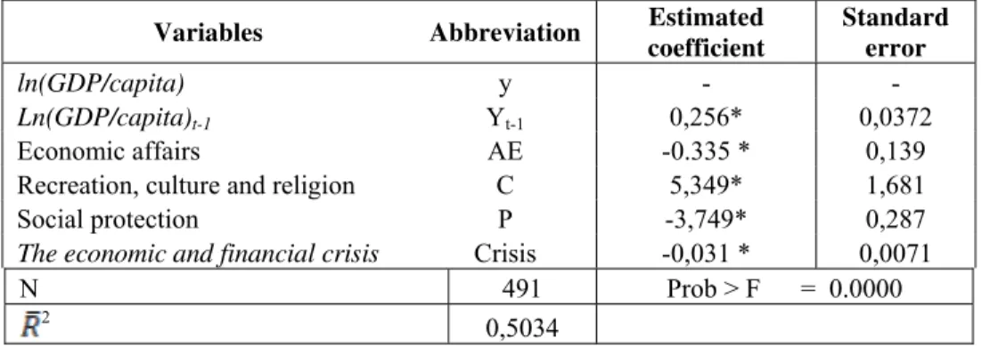
Variables Abbreviation Estimated
coefficient
Standard error
ln(GDP/capita) y - -
Ln(GDP/capita)t-1 Yt-1 0,256* 0,0372
Economic affairs AE -0.335 * 0,139
Recreation, culture and religion C 5,349* 1,681
Social protection P -3,749* 0,287
The economic and financial crisis Crisis -0,031 * 0,0071
N 491 Prob > F = 0.0000
2
0,5034
Legend: * 5% ** 10%
(Source: Stata v12)
Table 8. Results for the retested LSDV regression
There is also for the LSDV model a negative relationship between economic affairs and social protection and the economic growth. Thus, at 1 p.p. increase of economic affairs expenditure the GDP / capita decreases by 0.335 % and with negative 3.749% for increasing the social protection expenditure.
The expenditure for culture, recreation and religion are evolving in the same direction with the economic growth, so increase their growth by 1 percentage point to obtain 5.03% increase in GDP / capita.
In terms of dummy variables, it can also be said that the economic crisis has had an adverse effect on GDP per capita.
Next model used to determine the relationship between public spending and economic growth for the panel data is GMM - generalized method of moments
Roodman (2007) suggested that we need to verify the optimal lag and the tools/instruments that will be used for the GMM model. The tools consist of independent variables and / or dummy variables introduced in the model. To see the optimal lag we used the Sargan / Hansen test. For the instruments to be validated for
use in the model, H0 hypothesis must be rejected, so the χ2 value has to be greater
than 5%. Sargan test results are favourable and reject the null hypothesis only for a lag of eight.
Sargan test of overidentifying restrictions H0: overidentifying restrictions are valid
chi2(173) = 187.7923 Prob > chi2 = 0.2092 (Source: Stata v12)
Having established the lag of the Sargan test, we will analyse the results of the GMM model.
Variables Abbreviation Estimated
coefficient
Standard error
ln(GDP/capita) y - -
Ln(GDP/capita)t-1 Yt-1 0,914* 0,239
General public services S 0,195 0,200
Defence A -0.274 2,396
Public order and safety O -0,666 1,084
Economic affairs AE -0,906** 0,208
Environmental protection M 0,309** 1,996
Housing and community amenities L 0,245 0,809
Health H -0,425 0,630
Recreation, culture and religion C 4,276 2,375
Education E -1,553 1,655
Social protection P -4,256 0,361
N 461
Legend : * 5% ** 10%
(Source: Stata v12)
Table 10.Results for the GMM model
From the above table we can conclude that the significant variables that have an influence on economic growth are expenditure on economic affairs, environmental protection and social protection. Economic affairs and social protection have a negative effect on economic growth and environmental protection has a favourable effect.
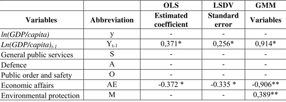
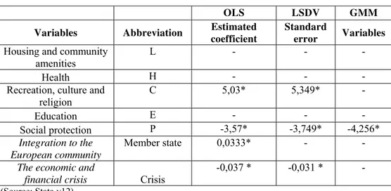
Following the three models used to determine the link between public spending and economic growth in the period 1991-2012, I have chosen to present the results summarized in the following table:
OLS LSDV GMM
Variables Abbreviation Estimated
coefficient
Standard
error Variables
ln(GDP/capita) y - - -
Ln(GDP/capita)t-1 Yt-1 0,371* 0,256* 0,914*
General public services S - - -
Defence A - - -
Public order and safety O - - -
Economic affairs AE -0.372 * -0.335 * -0,906**
OLS LSDV GMM
Variables Abbreviation Estimated
coefficient
Standard
error Variables Housing and community
amenities
L - - -
Health H - - -
Recreation, culture and religion
C 5,03* 5,349* -
Education E - - -
Social protection P -3,57* -3,749* -4,256*
Integration to the European community
Member state 0,0333* - -
The economic and
financial crisis Crisis
-0,037 * -0,031 * -
(Source: Stata v12)
Table 11.Summary of the three models used
The above table considers only the coefficients and the significance level for the explanatory variables that have an influence on the dependent variable. The OLS and LSDV models have the same types of public spending that influence economic growth, namely economic activities, culture, recreation and religion and social protection, the others being statistically insignificant.
Also in the GMM model social protection and economic affairs have considerable influence on economic growth, reducing it by 4.25% and 0.9%.
5. Conclusions
The present article analysed the correlation between public expenditure and economic growth in 30 European countries over the period between 1991 and 2012 using three econometric methods -OLS, LSDV and GMM. Statistical results for the 10 categories of expenditure have shown that economic affairs, environmental protection, recreation, culture and religion and social protection have a significant impact on economic growth. Also the recent economic crisis and the EU accession influenced the variation of GDP/capita.
Recreation, culture and religion and environmental protection have a positive effect on growth for the country sample.
6. References
Arellano, M. and Bover, O., 1995. Another look at the instrumental variable
estimation of error-components models. Journal of Econometrics, 68(1), pp. 29–51.
Arpaia, A. and Turrini, A., 2008. Government expenditure and economic growth in the EU: long-run tendencies and short-term adjustment. European Economy Economic Papers, No. 300, pp. 1-50.
Arusha, C., 2009. Government Expenditure, Governance and Economic Growth. Comparative Economic Studies, 51(3), pp. 401–418.
Barro, R. J. and Sala-i-Martin, X., 1995. Economic Growth. Cambridge: MIT Press, 25(3), pp. 159–163.
Barro, R. J., 1991. Economic growth in a cross section of countries. Quartely Journal of Economics, 106(2), pp. 407-443.
Blundell, R. and Bond, S., 1998. Initial conditions and moment restrictions in dynamic panel data models. Journal of Econometrics, 87(1), pp. 115–143. Bond, S. R., 2002. Dynamic panel data models: a guide to micro data methods and
practice. Portuguese Economic Journal, 1(2), pp. 141–162.
Brasoveanu, I., Brasoveanu, L.O. and Paun, C., 2008. Correlations Between Fiscal Policy And Macroeconomic Indicators In Romania. Theoretical and Applied Economics, Asociatia Generala a Economistilor din Romania - AGER, 11(528), pp. 51-59.
Devarajan, S., Swaroop, V. and Zou, H., 1996. The composition of public expenditure and economic growth. Journal of Monetary Economics, 37( 2), pp. 313–344.
Holzner, M., 2011. Inequality, growth and public spending in Central, East and
Southeast Europe. ECINEQ Working Papers 221, Society for the Study of
Economic Inequality.
Lamartina, S. and Zaghini, A., 2011. Increasing Public Expenditure: Wagner’s Law in OECD Countries. German Economic Review, 12(2), pp. 149–164.
Miyakoshi, T., Tsukuda, Y., Kono, T. and Koyanagi, M., 2010. Economic growth and public expenditure composition: Optimal adjustment using the gradient method. Japanese Economic Review, 61(3), pp. 320–340.
Roodman, B.D., 2007. The anarchy of numbers: Aid, development, and cross-country empirics. World Bank Economic Review, 21, pp. 255-277.
Wooldridge, J., 2002. Econometric Analysis of Cross Section and Panel Data, Cambridge: MIT press.