www.atmos-chem-phys.net/17/1161/2017/ doi:10.5194/acp-17-1161-2017
© Author(s) 2017. CC Attribution 3.0 License.
Probing the subtropical lowermost stratosphere and the tropical
upper troposphere and tropopause layer for inorganic bromine
Bodo Werner1, Jochen Stutz2, Max Spolaor2, Lisa Scalone1, Rasmus Raecke1, James Festa2, Santo Fedele Colosimo2, Ross Cheung2, Catalina Tsai2, Ryan Hossaini3, Martyn P. Chipperfield4, Giorgio S. Taverna4, Wuhu Feng5,
James W. Elkins6, David W. Fahey6, Ru-Shan Gao6, Erik J. Hintsa6,7, Troy D. Thornberry6,7, Free Lee Moore6,7, Maria A. Navarro8, Elliot Atlas8, Bruce C. Daube9, Jasna Pittman9, Steve Wofsy9, and Klaus Pfeilsticker1
1Institute of Environmental Physics, University of Heidelberg, Heidelberg, Germany
2Department of Atmospheric and Oceanic Science, University of California Los Angeles, Los Angeles, California, USA 3Lancaster Environment Centre, University of Lancaster, Lancaster, UK
4Institute for Climate and Atmospheric Science, School of Earth and Environment, University of Leeds, Leeds, UK 5National Centre for Atmospheric Science, School of Earth and Environment, University of Leeds, Leeds, UK 6NOAA Earth System Research Laboratory, Boulder, Colorado, USA
7Cooperative Institute for Research in Environmental Sciences (CIRES), University of Colorado, Boulder, Colorado, USA 8The Rosenstiel School of Marine and Atmospheric Science, University of Miami, Miami, Florida, USA
9School of Engineering and Applied Sciences, Harvard University, Cambridge, Massachusetts, USA
Correspondence to:Klaus Pfeilsticker (klaus.pfeilsticker@iup.uni-heidelberg.de) Received: 21 July 2016 – Published in Atmos. Chem. Phys. Discuss.: 19 September 2016 Revised: 20 December 2016 – Accepted: 5 January 2017 – Published: 25 January 2017
Abstract.We report measurements of CH4(measured in situ
by the Harvard University Picarro Cavity Ringdown Spec-trometer (HUPCRS) and NOAA Unmanned Aircraft System Chromatograph for Atmospheric Trace Species (UCATS) in-struments), O3(measured in situ by the NOAA dual-beam
ul-traviolet (UV) photometer), NO2, BrO (remotely detected by
spectroscopic UV–visible (UV–vis) limb observations; see the companion paper of Stutz et al., 2016), and of some key brominated source gases in whole-air samples of the Global Hawk Whole Air Sampler (GWAS) instrument within the subtropical lowermost stratosphere (LS) and the tropi-cal upper troposphere (UT) and tropopause layer (TTL). The measurements were performed within the framework of the NASA-ATTREX (National Aeronautics and Space Adminis-tration – Airborne Tropical Tropopause Experiment) project from aboard the Global Hawk (GH) during six deployments over the eastern Pacific in early 2013. These measurements are compared with TOMCAT/SLIMCAT (Toulouse Off-line Model of Chemistry And Transport/Single Layer Isentropic Model of Chemistry And Transport) 3-D model simulations,
aiming at improvements of our understanding of the bromine budget and photochemistry in the LS, UT, and TTL.
Changes in local O3(and NO2and BrO) due to transport
processes are separated from photochemical processes in in-tercomparisons of measured and modeled CH4and O3. After
excellent agreement is achieved among measured and simu-lated CH4and O3, measured and modeled [NO2] are found
TTL (i.e., when [CH4]≥1790 ppb), [Brinorgy ] is found to in-crease from a mean of 2.63±1.04 ppt for potential temper-atures (θ) in the range of 350–360 K to 5.11±1.57 ppt for
θ=390−400 K, whereas in the subtropical LS (i.e., when [CH4]≤1790 ppb), it reaches 7.66±2.95 ppt for θ in the
range of 390–400 K. Finally, for the eastern Pacific (170– 90◦W), the TOMCAT/SLIMCAT simulations indicate a net loss of ozone of −0.3 ppbv day−1 at the base of the TTL (θ=355 K) and a net production of+1.8 ppbv day−1in the upper part (θ=383 K).
1 Introduction
At present, bromine is estimated to be responsible for roughly one-third of the photochemical loss in global strato-spheric ozone (WMO, 2014). Past research has revealed that total stratospheric bromine (Bry) has (in 2013) four major sources or contributions: (1) CH3Br which is emitted by
nat-ural and anthropogenic sources, with a present contribution of 6.9 ppt to Bry, (2) four major halons (CClBrF2or
halon-1211; CBrF3 or halon-1301; CBr2F2 or halon-1202; and
CBrF2CBrF2or halon-2402), all emitted from anthropogenic
activities, with a present contribution of 8 ppt to Bry; (3) so-called very short-lived species (VSLS); and (4) inorganic bromine transported into the upper troposphere, e.g., previ-ously released from brominated VSLS and/or sea salt (e.g., Saiz-Lopez et al., 2004; Fernandez et al., 2014; Schmidt et al., 2016). This inorganic bromine is also partly trans-ported into the stratosphere. Together sources 3 and 4 are assessed to contribute 5 (2–8) ppt to stratospheric bromine (WMO, 2014). Previous assessments of total Bry and its trend revealed [Bry] levels of≈20 ppt (16–23 ppt) in 2011, which has been decreasing at a rate of −0.6 % yr−1 since the peak levels observed in 2000. This decline is consistent with the decrease in total organic bromine in the troposphere based on measurements of CH3Br, and the halons (WMO,
2014).
Estimates of stratospheric Bry essentially rely on two methods: first, the so-called organic (Brorgy ) method, where all bromine from organic source gases (SGs) found at the stratospheric entry level is summed (Wamsley et al., 1998; Pfeilsticker et al., 2000; Sturges et al., 2000; Brinckmann et al., 2012; Navarro et al., 2015). Second, total inorganic bromine (Brinorgy ) is inferred from atmospheric measurements (e.g., performed from the ground, aircraft, high-flying bal-loons, or satellites) of the most abundant Bry species, BrO, assisted by a suitable correction for the Brinorgy partition-ing inferred from photochemical modelpartition-ing (e.g., Pfeilsticker et al., 2000; Richter et al., 2002; Van Roozendael et al., 2002; Sioris et al., 2006; Dorf et al., 2006a, 2008; Hendrick et al., 2007; Theys et al., 2009, 2011; Rozanov et al., 2011; Par-rella et al., 2013; Stachnik et al., 2013). Further constraints on stratospheric Bry (range 20–25 ppt) were obtained by
satellite-borne measurements of BrONO2in the mid-infrared
(IR) spectral range at nighttime (Höpfner et al., 2009). While the organic method is rather precise for the measured species (accuracies are several tenths of a ppt), it suffers from the shortcoming of not accounting for any inorganic bromine (contribution 4) directly entering the stratosphere. Uncertain-ties in the inorganic method arise from uncertainUncertain-ties in mea-suring BrO as well as from modeling Brinorgy partitioning, of which the combined error amounts to±(2.5–4) ppt, depend-ing on the type of observation and probed photochemical regime.
Past in situ measurements of Brorgy were performed at different locations and seasons within the upper tropo-sphere, the tropical tropopause layer (TTL), and stratosphere. In the present context the most important were measure-ments performed within the TTL (for the definition of TTL, see Fueglistaler et al., 2009) over the Pacific from where most of the stratospheric air is predicted to originate (e.g., Fueglistaler et al., 2009; Aschmann et al., 2009; Hossaini et al., 2012b; Ashfold et al., 2012; WMO, 2014; Orbe et al., 2015). These include the measurements (a) by Schauffler et al. (1993, 1998, 1999), who found [VSLS]=1.3 ppt (con-tribution 3) at the tropical tropopause over the central Pacific (Hawaii) in 1996, (b) by Laube et al. (2008) and Brinckmann et al. (2012), with [VSLS]=2.25±0.24 ppt (range 1.4– 4.6 ppt) and [VSLS]=1.35 ppt (range 0.7–3.4 ppt) found within the TTL over northeastern Brazil in June 2005 and June 2008, respectively, and (c) most recently by Navarro et al. (2015), who found [VSLS]=2.96±0.42 and 3.27±0.49 ppt at 17 km over the tropical eastern and west-ern Pacific in 2013 and 2014, respectively. Information on contribution 3 was further corroborated by measurements performed in the upper tropical troposphere by Sala et al. (2014), who found [VSLS]=3.72±0.60 ppt in the upper tropical troposphere over Borneo in fall 2011, and by Wisher et al. (2014), who inferred [VSLS]=3.4±1.5 ppt for the CARIBIC (Civil Aircraft for the Regular Investigation for the Atmosphere Based on an Instrument Container) flights from Germany to Venezuela and Colombia during 2009– 2011, Germany to South Africa during 2010 and 2011, and Germany to Thailand and Kuala Lumpur, Malaysia, during 2012 and 2013.
stratosphere, while (b) Liang et al. (2014) estimated that up to 8 ppt of VSLS bromine may enter the base of the TTL at 150 hPa, whereby the VSLS emissions from the tropical Indian Ocean, the tropical western Pacific, and off the Pa-cific coast of Mexico are suspected to be most relevant, and finally (c) the Community Atmosphere Model with Chem-istry (CAM-Chem) modeling performed within the study of Navarro et al. (2015), which indicates that over the east-ern and westeast-ern Pacific contributions 3 and 4 (called [VSLS + Brinorgy ] in the study) amount to 6.20 ppt (range 3.79– 8.61 ppt) and 5.81 ppt (range 5.14–6.48 ppt), respectively.
Using the inorganic method, contributions 3 and 4 have been indirectly estimated from BrO mea-sured at the ground, high-flying balloons, or satel-lites (e.g., Pfeilsticker et al., 2000; Richter et al., 2002; Van Roozendael et al., 2002; Sioris et al., 2006; Dorf et al., 2006b; Dorf et al., 2008; Hendrick et al., 2007; Theys et al., 2009; Theys et al., 2011; Rozanov et al., 2011; Parrella et al., 2013; Stachnik et al., 2013). All together these studies pointed to a range between 3 and 8 ppt with a mean of 6 ppt for contributions 3 and 4. The most direct information on contributions 3 and 4 come from the studies of Dorf et al. (2008), WMO (2011), and Brinckmann et al. (2012). They inferred 1.25±0.16 ppt (very short lived – source gases, VSL-SGs, contribution 3) +4.0±2.5 ppt (product gases, PGs, contribution 4)=5.25±2.5 ppt (contri-butions 3 and 4) and 2.25±0.24 ppt (VSL-SGs, contribution 3) +1.68±2.5 ppt (PGs, contribution 4)=3.98±2.5 ppt (contributions 3 and 4) from two balloon-borne soundings performed in the TTL and stratosphere over northeastern Brazil during the dry season in 2005 and 2008, respectively. The inferred bromine was thus often larger than [VSLS] inferred using the organic method (contribution 3), indicat-ing that variable amounts of Brinorgy (i.e., several parts per trillion) are directly transported from the troposphere into the stratosphere (contribution 4).
Based on these findings, Saiz-Lopez et al. (2012) and Hos-saini et al. (2015) provided evidence for the efficiency of short-lived halogens to influence climate through depletion of lower-stratospheric ozone (for contribution 3) but without explicitly considering the effect of inorganic bromine read-ily transported across the tropical tropopause (i.e., contribu-tion 4). They concluded that VSLS bromine alone exerts a 3.6 times larger ozone radiative effect than is due to long-lived halocarbons when normalized to their halogen content. Moreover the benefit for ozone and UV radiation due to the declining stratospheric chlorine and bromine since the imple-mentation of the Montreal protocol was quantified in a recent study by Chipperfield et al. (2015). Finally, in a recent study Fernandez et al. (2016) pointed out that bromine from contri-bution 3 and 4 contributes about 14 % to the formation of the present Antarctic ozone hole, in particular at its periphery. Further, they suggests a large influence of biogenic bromine on the future Antarctic ozone layer.
The present paper reports measurements of BrO (and NO2,
O3, CH4, and the brominated source gases) made during the
ATTREX (Airborne Tropical Tropopause Experiment) de-ployments of the NASA Global Hawk into the lowermost stratosphere (LS), upper troposphere (UT), and TTL of the eastern Pacific in early 2013. Corresponding data collected during the western Pacific deployments in early 2014 will be reported in a forthcoming paper, primarily since most of the 2014 measurements were performed under TTL cirrus-affected conditions, for which the interpretation of UV– visible (UV–vis) spectroscopic measurements is not straight-forward (see below). The present paper further addresses the amount of inorganic bromine found in the TTL and its trans-port into the lowermost tropical stratosphere (contribution 4), together with the implications for ozone.
Our study accompanies those of Navarro et al. (2015) and Stutz et al. (2016). While Stutz et al. (2016) discusses the instrumental details and the methods employed to remotely measure BrO, NO2, and O3, the study of Navarro et al. (2015)
reports the Global Hawk Whole Air Sampler (GWAS) mea-surements of CH3Br (contribution 1), the halons
(contribu-tion 2), and the brominated VSLS (contribu(contribu-tion 3) analyzed in whole-air samples, which were simultaneously taken from aboard the NASA Global Hawk over the eastern and western Pacific during the 2013 and 2014 deployments, respectively. The paper is organized as follows. Section 2 briefly de-scribes all key methods used in the present study. Section 3 discusses the measurements along with some (necessary) data reduction. In Sect. 4, the major observations are pre-sented and they are compared with previous BrO measure-ments and our modeling results, along with their implica-tions for the amount of inorganic bromine present within the TTL. Further implications of our measurements for the pho-tochemistry of bromine and ozone within the TTL and low-ermost subtropical stratosphere are discussed. Section 5 con-cludes the study.
2 Methods
The instruments of the NASA-ATTREX package most im-portant for the present study consist of a fast UV photome-ter for measurement of ozone (Gao et al., 2012), a gas chro-matograph (Unmanned Aircraft System Chrochro-matograph for Atmospheric Trace Species – UCATS; Wofsy et al., 2011, and Moore et al., 2003) as well as a Picarro instrument (Har-vard University Picarro Cavity Ringdown Spectrometer – HUPCRS; Crosson, 2008; Rella et al., 2013; Chen et al., 2013) to measure CH4, CO2, and CO, a whole-air sampler
(GWAS; Schauffler et al., 1998, 1999) to analyze a large suite of stable trace gases, and a three-channel scanning limb mini-DOAS (differential optical absorption spectroscopy) instru-ment for spectroscopic detection of O3, NO2, BrO, OClO,
IO, O4, O2, H2Ovapor, H2Oliquid, and H2Osolidin the UV–vis–
Stutz, 2008; Kritten et al., 2010, 2014; Kreycy et al., 2013; Stutz et al., 2016).
All instruments, techniques, methods, and tools are briefly described in the following.
2.1 DOAS measurements of O3, NO2, and BrO
The mini-DOAS instrument is a UV–vis–near-IR three-channel optical spectrometer by which scattered skylight re-ceived from limb direction and direct sunlight can be an-alyzed for O3, NO2, and BrO (as well as for some other
species; see above). Since the instrument and retrieval meth-ods are described in detail in the accompanying paper by Stutz et al. (2016) (for further details, see Table 2 therein), only some key elements of the data analysis are described here.
The post-flight analysis of the collected data for the de-tection of O3, O4, NO2, and BrO and concentration retrieval
include (a) the spectral retrieval of the targeted gases using the DOAS method (Platt and Stutz, 2008) (for the DOAS settings, see Table 4 in Stutz et al., 2016), (b) forward ra-diative transfer (RT) modeling of each observation using the Monte Carlo model McArtim (Monte Carlo Atmospheric Ra-diative Transfer Inversion Model; Deutschmann et al., 2011; for further details, see Sect. 2.6), and (c) for the concentra-tion and profile retrieval either the nonlinear optimal estima-tion (Rodgers, 2000) or the novel x gas scaling technique (for details, see Sect. 4.2. and 4.3 in Stutz et al., 2016). Typi-cal errors are±5 ppb for O3,±15 ppt for NO2, and±0.5 ppt
for BrO, to which possible systematic errors in the individ-ual absorption cross section need to be added. These are for O3-UV±1.3 %, O3-vis±2 %, NO2±2 %, and BrO±10 %
(for more details on the error budget, see Stutz et al., 2016).
2.2 In situ measurements of O3
The NOAA-2 polarized O3 photometer (Gao et al., 2012)
is a derivative of the dual-beam, unpolarized, UV absorp-tion technique described by Proffitt and McLaughlin (1983). Briefly, the ambient and O3-free air flow is alternately
di-rected into two identical 60 cm long absorption cells. The 253.7 nm UV light from a mercury lamp is split into two beams that are each directed into one of the absorption cells. Since O3strongly absorbs 253.7 nm photons, the UV beam
passing through the cell containing ambient ozone is attenu-ated more than the beam passing through the cell contain-ing O3-free air. Knowing the O3 absorption cross section
(σ (O3)) and the absorption path length (L), the O3 partial
pressure (p(O3)) in the ambient air can be derived using
Beer’s law.
The instrument has a fast sampling rate (2 Hz at<200 hPa, 1 Hz at 200 to 500 hPa, and 0.5 Hz at ≥500 hPa), high ac-curacy (3 % excluding operation in the 300–450 hPa range, where the accuracy may be degraded to about 5 %), and excellent precision (1.1×10¹⁰ O3molecules cm−3 at 2 Hz,
which corresponds to 3.0 ppb at 200 K and 100 hPa or 0.41 ppb at 273 K and 1013 hPa). The size (36 L), weight (18 kg), and power (50–200 W) make the instrument suitable for many unmanned aerial vehicle systems and other airborne platforms. In-flight and laboratory intercomparisons with ex-isting O3instruments have shown that measurement accuracy
(3 %) is maintained in flight.
2.3 CH4measurements by UCATS
The UCATS measures atmospheric methane (CH4) on one
gas chromatographic channel along with hydrogen (H2) and
carbon monoxide (CO) once every 140 s. UCATS has two chromatographic channels with electron capture detectors (ECDs), two ozone (O3) ultraviolet absorption
spectrome-ters, and a water vapor (H2O) tunable diode laser absorption
spectrometer (TDLAS). The details of the CH4
chromatogra-phy are similar to those on balloon and airborne instruments described in Moore et al. (2003) and Elkins et al. (1996). The addition of∼100 ppm of nitrous oxide to the make-up line of the ECD enhances the sensitivity to H2, CO, and CH4
(Elkins et al., 1996, and Moore et al., 2003). The separa-tion of these gases in air is accomplished with a pre-column of Unibeads (2 m×2 mm diameter), and a main column of molecular sieve 5A (0.7 m×2.2 mm diameter) at∼110◦C (Moore et al., 2003). The precision of the CH4
measure-ment during ATTREX was±0.5 % and is calibrated during flight with a secondary standard after every three ambient air measurements. Instrumental drift is corrected between the standard injections. UCATS measurements are trace-able to the WMO Central Calibration Laboratory (CCL) and are on the CH4 WMO X2004A scale (Dlugokencky et al.,
2005, with updates given at http://www.esrl.noaa.gov/gmd/ ccl/ch4_scale.html).
2.4 CH4measurements by HUPCRS
The HUPCRS consists of a G2401-m Picarro gas ana-lyzer (Picarro Inc., Santa Clara, CA, USA) repackaged in a temperature-controlled pressure vessel, a separate calibra-tion system with two multi-species gas standards, and an external pump and pressure control assembly designed to allow operation at a wide range of altitudes. The Picarro analyzer uses wavelength-scanned cavity ringdown spec-troscopy (WS-CRDS) technology to make high-precision measurements of greenhouse gases (Crosson, 2008; Rella et al., 2013; Chen et al., 2013). HUPCRS reports concen-trations of CO2, CH4, and CO every∼2.2 s and the data are
averaged to 10 s. In-flight precision for CH4 is 0.2 ppb in
10 s.
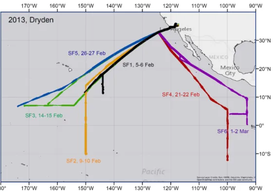
Figure 1.Overview of the NASA Global Hawk ATTREX flights conducted from Dryden in 2013. The thickness of the lines corresponds to flight altitudes, where the thinnest line is for an altitude of around 14 km and the thickest line for around 18 km.
keep the cavity at 140±0.02 Torr and 45±0.0005◦C in or-der to stabilize the spectra. The injected light is blocked pe-riodically, and when blocked, the exponential decay rate of the light intensity is measured by a photodetector. The de-cay rate depends on loss mechanisms within the cavity such as mirror losses, light scattering, refraction, and absorption by a specific analyte. A sequence of specific wavelengths for each molecule is injected into the cavity in order to recon-struct the absorption spectra. A fit to the spectra is performed in real time and concentrations are derived based on peak height. High-altitude sampling (i.e., very low pressure and temperature) necessitated transferring the core components of the Picarro analyzer to a sealed tubular pressure vessel, which is maintained at 35◦C and 760 Torr. The analyzer’s components are isolated from the pressure vessel to provide vibration damping and decoupling from deformations in the pressure vessel caused by external pressure changes.
The sampling strategy for HUPCRS consists of bringing in air through a rear-facing inlet, filtered by a 2 µm Zefluor membrane, and dehydrating this air by flowing it through a multi-tube Nafion dryer followed by a dry-ice cooled trap prior to entering the Picarro analyzer. A choked upstream Teflon-lined diaphragm pump delivers ambient air to the an-alyzer at 400 Torr, regardless of aircraft altitude, via a flow bypass. A similar downstream pump, with an inlet pressure of 10 Torr, facilitates flow through the analyzer at high alti-tude and ensures adequate purging of the Nafion drier. Mea-surement accuracy and stability are monitored by replacing ambient air with air from two NOAA-traceable gas standards
(low- and high-span) for a total of 4 min every 30 min. These standards are contained in 8.4 L carbon fiber wrapped alu-minum cylinders and housed in a temperature-controlled en-closure. The total weight of the package is 97 kg.
2.5 The Global Hawk Whole Air Sampler
The GWAS is a modified version of the Whole Air Sam-pler used on previous airborne campaigns (Heidt et al., 1989; Schauffler et al., 1998, 1999; Daniel et al., 1996). Briefly, the instrument consists of 90 custom-made Silonite-coated (Entech Instruments, Simi Valley, CA) canisters of 1.3 L, controlled with Parker Series 99 solenoid valves (Parker-Hannifin, Corp., Hollis, NH). Two metal bellows compres-sor pumps (Senior Aerospace, Sharon, MA) allow the flow of ambient air through a custom inlet at flow rates rang-ing from 2 to 8 standard L min−1, depending on altitude. The manifold and canister module temperatures are controlled to remain within the range of 0–30◦C. GWAS is a fully
18 km. The samples are analyzed using a high-performance gas chromatograph (Agilent Technology 7890A) and mass spectrometer with mass selective, flame ionization and elec-tron capture detectors (Agilent Technology 5975C). Sam-ples are concentrated on an adsorbent tube at −38◦C with a combination of cryogen-free automation and thermal des-orber system (CIA Advantage plus UNITY 2, Markes Inter-national). The oven temperature profile is−20◦C for 3 min, then 10◦C min−1to 200◦C, and 200◦C for 4 min for a total analysis time of 29 min. Under these sampling conditions the precision is compound/concentration dependent and ranged from≤2 to 20 %. Calibration procedures as well as mixing ratio calculations are described elsewhere (Schauffler et al., 1999).
During ATTREX 2013 the whole-air sampler measured a variety of organic trace gases, including non-methane hy-drocarbons, CFCs, HCFCs, methyl halides, solvents, or-ganic nitrates, and selected sulfur species. For this work a range of long- and short-lived organic bromine gases are measured, including CH3Br, CH2Br2, CH2BrCl, CHBrCl2,
CHBr2Cl, CHBr3, and halon-1211 (CBrClF2) and halon
2402 (C2Br2F4). Halon-1301 (CBrF3) is not measured and
a constant value of 3.3 ppt is used to account for the bromine content from this compound.
2.6 Radiative transfer modeling
The measured limb radiances of the mini-DOAS instrument are modeled in spherical 1-D and in selected cases in 3-D, using version 3.5 of the Monte Carlo RT model McArtim (Deutschmann et al., 2011). The model’s input is chosen ac-cording to the on-board measured atmospheric temperatures and pressures, including climatological low-latitude aerosol profiles from Stratospheric Aerosol and Gas Experiment III (SAGE III) (https://eosweb.larc.nasa.gov/project/sage3/ sage3_table), and lower-atmospheric cloud covers as indi-cated by the cloud physics lidar measurements made from aboard the Global Hawk (GH; see http://cpl.gsfc.nasa.gov/). In the standard run, the ground (oceanic) albedo is set to 0.07 in UV and 0.2 in the visible spectral range. The RT model is further fed with the actual geolocation of the GH, solar zenith, and azimuth angles as encountered during each measurement, the telescopes azimuth and elevation angles, as well as the field of view (FOV) of the mini-DOAS telescopes. Figure 5 in Stutz et al. (2016) displays one example of an RT simulation for limb measurements at 18 km altitude. The simulation indicates that correctly accounting for the Earth’s sphericity, the atmospheric refraction, cloud cover, ground albedo, etc., is relevant for the interpretation of UV–vis–near-IR limb measurements performed within the middle atmo-sphere (Deutschmann et al., 2011). Even though the three (UV–vis–near-IR) mini-DOAS spectrometers are not radio-metrically calibrated on a absolute scale, past comparison exercises of measured and McArtim modeled limb radiance provide confidence in the quality of the RT simulations (see,
e.g., Figs. 5 and 6 in Deutschmann et al., 2011, and Fig. 2 in Kreycy et al., 2013).
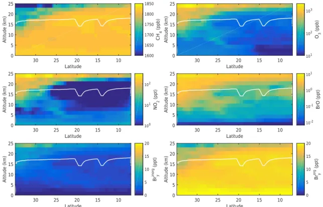
For the simulations of the trace gas absorptions mea-sured in limb direction, the RT model is further fed with TOMCAT/SLIMCAT-simulated curtains of the targeted gases simulated along the GH flight paths (see Sect. 2.7). In the RT simulations [BrO] is set to 0.5 ppt near the ground, where TOMCAT/SLIMCAT predicts lower BrO concentra-tions (see Fig. 2 middle right panel), in agreement with the findings discussed in Stutz et al. (2016) and the recent study of Schmidt et al. (2016).
2.7 Photochemical modeling
For the interpretation of our measurements, we use sim-ulations of the TOMCAT/SLIMCAT 3-D chemical trans-port model (CTM; Chipperfield, 1999, 2006). More specifi-cally, the simulations are used for intercomparison with mea-sured photochemical species, for assessment of the budget of Brinorgy , and for sensitivity studies on the impact of our mea-surements on the photochemistry of bromine and ozone in the subtropical UT–LS, tropical UT, and TTL.
For the present study, the TOMCAT/SLIMCAT model is driven by meteorology from the ECMWF ERA-interim reanalyses (Dee et al., 2011). The reanalyses are used for large-scale winds and temperatures as well as convective mass fluxes (Feng et al., 2011). The model has a detailed stratospheric chemistry scheme with kinetic and photochemical data taken from JPL-2011 (Sander et al., JPL-2011), with recent updates. The model chemical fields are constrained by specified time-dependent surface mixing ratios. For the brominated species, the following surface mixing ratios of stratospheric-relevant source gases are assumed: [CH3Br]=6.9 ppt;
[halons]=7.99 ppt; [CHBr3]=1 ppt; [CH2Br2]=1 ppt; and 6 [CHClBr2,CHCl2Br,CH2ClBr,etc.]=1 ppt of Br.
observa-Latitude 10 15 20 25 30 Altitude (km) 0 5 10 15 20 25 O3 (ppb) 101 102 103 Latitude 10 15 20 25 30 Altitude (km) 0 5 10 15 20 25 BrO (ppt) 10-2 10-1 100 101 Latitude 10 15 20 25 30 Altitude (km) 0 5 10 15 20 25 NO 2 (ppt) 100 101 102 Latitude 10 15 20 25 30 Altitude (km) 0 5 10 15 20 25 CH 4 (ppb) 1600 1650 1700 1750 1800 1850 Latitude 10 15 20 25 30 Altitude (km) 0 5 10 15 20 25 Bry inorg (ppt) 0 5 10 15 20 Latitude 10 15 20 25 30 Altitude (km) 0 5 10 15 20 25 Bry org (ppt) 0 5 10 15 20
Figure 2.TOMCAT/SLIMCAT predictions of mixing ratio curtains of CH4(upper left), O3(upper right), NO2(middle left), BrO (middle
right), Brinorgy (bottom left), and Brorgy (bottom right) for the sunlit part of SF3-2013 (14 February 2013). Note the different color scale ranges.
The white line is the flight trajectory of the Global Hawk. For better visibility, the simulated mixing ratios are shown for the altitude range 0–25 km, although the TOMCAT/SLIMCAT simulations cover the range of 0–63 km altitude.
tions of AGAGE (Advanced Global Atmospheric Gases Ex-periment; https://agage.mit.edu/) and NOAA, which reflect recent variations in its growth rate.
The standard model run (no. 583) is initialized in 1979 and spun-up for 34 years at low horizontal resolution (5.6◦×5.6◦) and with 36 unevenly spaced sigma-pressure
vertical levels in the altitude range 0–63 km. Output from 1 January 2013 is interpolated to a high horizontal resolu-tion (1.2◦×1.2◦), and the simulation continued over the AT-TREX campaign period using this resolution. The model out-put is sampled online along the Global Hawk flight tracks for direct comparison with the observations. Two further high-resolution sensitivity experiments are performed from 1 Jan-uary 2013 onwards. In run no. 584, the ratio of the photoly-sis frequency of BrONO2and the three-body association rate
reaction coefficient kBrO+NO2 is increased by a factor 1.75
(e.g., Kreycy et al., 2013). In run no. 585 the second-order rate reaction coefficient kBr+O3 is set to the upper limit of its
uncertainty range (Sander et al., 2011).
For all model levels and for the time resolution (∼30 s) of the mini-DOAS measurements, “curtains” of the targeted gases along the flight track are stored (see, e.g., Fig. 6 in Stutz et al., 2016, and Fig. 2 of our present study). They are im-ported into the RT model McArtim for further forward sim-ulations of the observations, and measurement-versus-model intercomparison studies. The inclusion of simulated
TOM-CAT/SLIMCAT curtains in our study is particularly neces-sary for (a) the retrieval of absolute concentrations using the O3-scaling technique (see Stutz et al., 2016, Sect. 4.3), (b)
es-timate of errors and retrieval sensitivities to various parame-ters (see Sect. 4.4 and the Supplement to Stutz et al., 2016), (c) the separation of dynamical and photochemical processes in the interpretation of our data, (d) sensitivity tests for the assumed kinetic data, and (e) the assessment of total Brinorgy (see Sect. 4).
Finally, details of how the loss in ozone is calculated is provided in Appendix Sect. A.
3 Measurements and data reduction
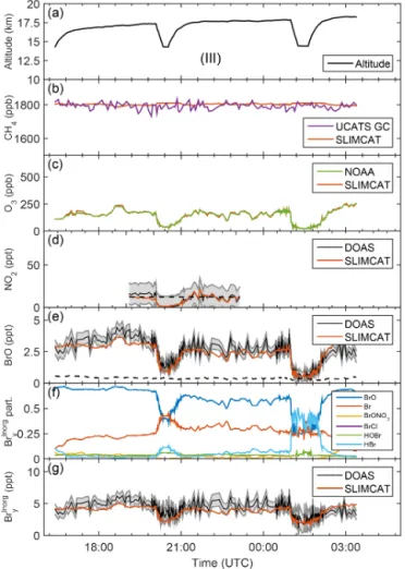
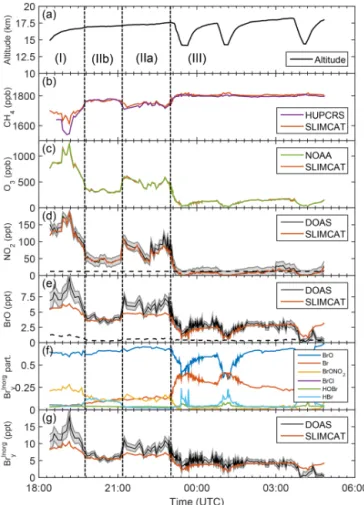
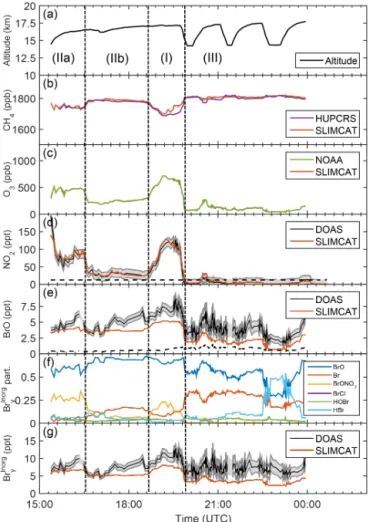
Figure 3. Panel (a) shows the time–altitude trajectory of the sunlit part of the GH flight track (SF1-2013) on 4–5 Febru-ary 2013 (SF1-2013). Panels (b)–(e) show intercomparisons of TOMCAT/SLIMCAT-simulated fields with observations of(b)CH4 (UCATS), (c)O3(NOAA),(d) NO2 (mini-DOAS), and (e)BrO (mini-DOAS). The grey-shaded error bars of the mini-DOAS NO2 and BrO measurements include all significant errors, i.e., the spec-tral retrieval error, the error due to a contribution to the slant ab-sorption from above the aircraft and from the troposphere, and the absorption cross section uncertainty. Panel (f) shows the SLIM-CAT modeled Brypartitioning for the standard run no. 583. Panel
(g)shows a comparison of inferred and modeled Brinorgy , including
the uncertainty as a grey band.
instrument package, the flights, and some results of the col-lected data can be found in Jensen et al. (2013, 2015), as well as on the project’s website https://espo.nasa.gov/missions/ attrex/content/ATTREX.
In February and March 2013, the NASA-ATTREX flights of the Global Hawk were strongly biased with respect to the sampled air masses, mostly because the scientific interest was primarily put on probing the TTL over the eastern Pacific for aerosols and cirrus cloud particles during the convective season rather than for the photochemistry of bromine in the LS, UT, and TTL (see Fig. 1). Therefore, and due to
opera-Figure 4.Same as Fig. 3 but for the research flight on 9–10
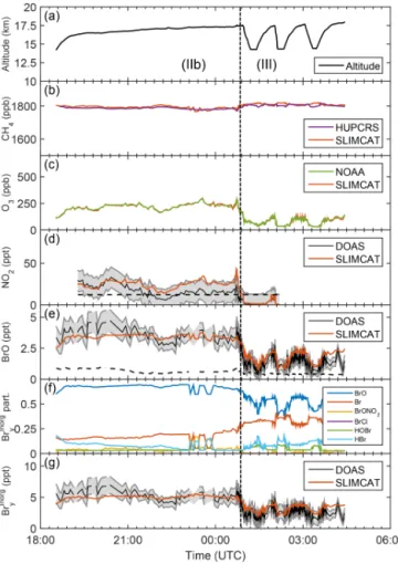
Febru-ary 2013 (SF2-2013). The dashed vertical lines in Figs. 4–9 sep-arate different atmospheric regimes: (I) is the extratropical lower-most stratosphere; (IIa, IIb, etc.) are different mixing regimes of air from the extratropical lowermost stratosphere; and (III) is from the tropical tropopause layer.
tional reasons, typical flight patterns extended from Dryden, California, in a southerly or southwesterly direction during daytime until a turn-point was reached, and the back leg to Dryden in a northeasterly direction occurred during the night when the mini-DOAS instrument could not take measure-ments. The dives were mostly performed within the TTL and occasionally within the subtropical lowermost stratosphere during the return legs at night but not during the outgoing daytime legs. Finally the landings at Dryden were scheduled for the early local morning, mostly due to operational con-straints. Therefore, no profiles of the targeted species could be obtained in the subtropical lowermost stratosphere during the daytime, but a large number were obtained within the UT and TTL.
should be where the subtropical jet is located. However, since we do not infer dynamical parameters (such as the potential vorticity) from our data, we conveniently define the bound-ary according to proxies for (a) different air mass ages (i.e.,
[CH4]concentrations≤1790 ppb are labeled subtropical and
[CH4]≥1790 ppb are labeled tropical) and (b)
photochem-ical regimes (i.e., [O3] is subtropical when [O3]≥150 ppb
and TTL when [O3]≤150 ppb), which we find suitable from
a visual inspection of our data (see below).
As mentioned above and outlined in detail in the study of Stutz et al. (2016), the processing of the mini-DOAS data included (a) spectral retrieval of the targeted gases from the mini-DOAS measurements (Sect. 2.1), (b) forward modeling of the RT for each measured spectrum (Sect. 2.6), and (c) either applying optimal estimation or the novel x gas scal-ing technique (see Sect. 4.1 and 4.2 in Stutz et al., 2016). Comprehensive sensitivity simulations indicated that optical estimation based on constraints inferred from measured O4
and/or relative radiance would not result in the desired error range (Stutz et al., 2016, Sect. 4.2). Therefore, we decided to apply thex gas scaling technique (Stutz et al., 2016, and Raecke, 2013) with x being ozone measured in situ by the NOAA-2 O3photometer (see Sect. 2.2).
The O3-scaling technique makes use of the in situ O3
mea-sured by the NOAA instrument (Gao et al., 2012) and the limb-measured O3total slant column amounts (SCDO3)
ei-ther monitored in the UV (for the retrieval of BrO in the 343–355 nm wavelength band) or visible wavelength range (for the retrieval of NO2in the 424–460 nm wavelength band;
see Eq. 12 in Stutz et al., 2016). Here the ratio of the mea-sured slant column and SCDO3/[O3] measured in situ can
be regarded as a proxy for the (horizontal) light path length over which the absorption is collected. In fact, in the paper of Stutz et al. (2016), it is argued that the so-calledα fac-tors account for the fraction of the absorption of the scal-ing gasx (e.g.,x=O3in our study) picked up on the
hor-izontal light paths ahead of the aircraft relative to the total measured absorption. The sensitivity study on the αfactors presented in Stutz et al. (2016) (e.g., in the Supplement) in-dicates that for the targeted gases, uncertainties in αfactor ratios due to assumptions regarding the RT (for example due to Mie scattering by aerosols and clouds) mostly cancel out, while uncertainties in the individual profile shapes of the tar-geted and scaling gas are most relevant for the errors of the inferred gas concentrations. Therefore, in the present study, profile shapes of the targeted and scaling gas predicted by the TOMCAT/SLIMCAT CTM are used in the RT calcula-tions, aiming at the calculation of theαfactors. The uncer-tainties in the profile shapes (assumed to be of the order of the altitude adjustment of the CH4and O3 curtains, which
are typically much smaller than the altitude grid spacing in the SLIMCAT/TOMCAT simulations) are then carried over to calculate the overall errors, as discussed in Sect. 4.4 of the Stutz et al. (2016) study.
It should be noted that for the flight on 21 February 2013 (SF4-2013), the DOAS retrieval is much less robust than for all the other flights, most likely because the Fraunhofer ref-erence spectra (taken via a diffuser) are affected by tempo-rally changing residual structures likely due to ice deposits or some other residues on the entrance diffuser. Therefore, the data of this flight are not analyzed in detail, but they are only reported for completeness here.
Finally, in our analysis only those data which are taken at a solar zenith angle (SZA) ≤88◦ are considered be-cause for increasing SZAs the received skylight radiance re-quires increasingly longer signal integration times (longer than the standard integration time, which is 30 s) and are thus averaged over longer distances ahead of the aircraft. Moreover, as the SZA increases, the skylight is expected to traverse an increasingly inhomogeneous curtain of the probed radicals (e.g., see Figs. 5 and 6 in Stutz et al., 2016). As a consequence, the spatial grid of TOMCAT/SLIMCAT (1.2×1.2◦) on which the photochemistry is simulated ap-peared too coarse for a useful interpretation of our measure-ments at large SZAs. Therefore, for a tighter interpretation of our data, a model with higher spatial resolution than pro-vided by TOMCAT/SLIMCAT would be required. Such an approach is for example followed in the balloon-borne stud-ies of Harder et al. (2000), Butz et al. (2009), Kreycy et al. (2013), and others. However, since both processes are likely to increase the error of our analysis and since large SZA (≥88◦) measurements only constitute a minor part of all measurements, we refrain from this much more complicated approach.
4 Results and discussion
In this section we first discuss how our mini-DOAS measure-ments of O3, NO2, and BrO, as well as of CH4(from UCATS
4.1 Comparison with TOMCAT/SLIMCAT predictions
Figures 3 to 8 provide overviews on the measured data to-gether with the TOMCAT/SLIMCAT modeled Brinorgy parti-tioning (panels f) and inferred total Brinorgy (panels g) as a function of universal time for each flight. The modeled val-ues are obtained by linear interpolation of the curtain data (see Fig. 2) to the exact altitude of the GH.
The panels b and c of Figs. 3 to 8 show comparisons of measured and modeled CH4and O3mixing ratios. Here the
measured and modeled species closely agree within the given error bars after the modeled curtains are altitude-shifted (i.e., interpolated) by the same amount until measured and mod-eled O3agree (for details, see Stutz et al., 2016). It is
note-worthy that in most cases the altitude adjustment is less than the grid spacing of TOMCAT/SLIMCAT (about 1 km in the TTL), thus mostly accounting for the altitude mismatches of the actual cruise altitude of the Global Hawk and the model output rather than indicating deficits of the model in prop-erly predicting the vertical transport. The astonishingly good agreement achieved between measured and modeled CH4,
and O3 lends confidence that the altitude-adjusted
TOM-CAT/SLIMCAT model fields reproduce the essential dynam-ical and photochemdynam-ical processes of the probed air masses well. The quality of the dynamical simulations are further tested by comparing modeled and measured O3as a function
of CH4(Fig. 9). For all flights the agreement of the observed
and modeled O3vs. CH4correlation is reasonably good,
ex-cept for flights SF1-2013 and SF2-2013, where the UCATS measured CH4 scatters around the simulated CH4
concen-trations. This scatter is most likely due to precision errors of UCATS rather than reflecting the real behavior of the at-mosphere. Evidence for this conclusion is provided from the CH4comparisons for SF3-2013 and SF6-2013, in which the
HUPCRS CH4data are taken; these data do not show such
scatter and compare reasonably well with the model predic-tions.
Panels d of Figs. 3 to 8 compare measured and modeled NO2. Overall, the measured (and modeled) NO2
concentra-tions meet the expectaconcentra-tions with respect to NO2partitioning
and total NOx(=NO+NO2+NO3) abundances in the LS,
UT, and TTL over the pristine Pacific. Elevated NO2
concen-trations (range 70 to 170 ppt) are measured within the sub-tropical lowermost stratosphere, where aged air masses are probed, as indicated by depleted CH4concentrations and
el-evated O3 concentrations (and presumably decreased N2O
concentrations). Note that N2O is the primary source for
stratospheric NOx, and in the stratosphere CH4and N2O
de-struction processes closely follow each other (e.g., Michelsen et al., 1998; Ravishankara et al., 2009). Very low NO2
con-centrations (≤30 ppt) are detected within the UT and TTL, indicating that the analyzed air does not originate from re-cently polluted or lightning-affected regions. Further, the modeled NO2concentrations (red line in panel d) are found
Figure 5.Same as Fig. 3 but for the research flight on 14–15
Febru-ary 2013 (SF3-2013).
to fall into the given range of errors in the measured NO2
concentrations. This finding strongly indicates that the NOx and NOy (=NOx, N2O5, HONO3, HO2NO2, etc.) budget
and photochemistry of the LS, UT, and TTL are reproduced well in the TOMCAT/SLIMCAT simulations and that overall the O3-scaling technique works well for NO2.
4.2 Comparison of measured and model organic bromine
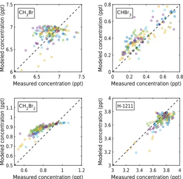
Before measured and modeled BrO can be compared quan-titatively, it is necessary to compare the measured amounts of different brominated source gases with the model predic-tions (Fig. 10). For the assumed (constant) surface mixing ra-tios (see Sect. 2.7), measured and modeled CH3Br (upper left
panel), CHBr3(upper right panel), and all other halons, for
example H1211 (lower right panel), compare well, even if the data are scattered from flight to flight. For CH2Br2, however,
TOMCAT/SLIMCAT run no. 583 underpredicts the observed mixing ratio for high concentrations (by 0.1 ppt) and over-predicts it by up to 0.2 ppt for low concentrations (lower left panel). This is most likely due to an assumed a surface con-centration that is too low (1 ppt), variable mixing ratios at the surface not being correctly considered in the model, and/or errors in the atmospheric lifetime by reactions of CH2Br2
with OH radicals in the model (e.g., Mellouki et al., 1992; Ko et al., 2013; WMO, 2014).
The flight-to-flight and sample-to-sample scatter in CH3Br
and CHBr3is mostly due to different source regions of the air
masses probed during SF1-2013 to SF6-2013. This implies a spatially (and possibly time-dependent) varying source strength of the brominated natural source gases (e.g., Hos-saini et al., 2013; Ziska et al., 2013). In the present version of the TOMCAT/SLIMCAT simulations, this scatter intro-duces an estimated uncertainty of±0.8 ppt into Brorgy , and potentially into the inferred Brinorgy available in the TTL. The systematic underprediction of 0.1 ppt at high CH2Br2
con-centrations and its overly long lifetime in the TTL leading to CH2Br2concentrations in the model that are too large for
old air (by up to 0.2 ppt). Consequently, the model underpre-dicts Brinorgy by an additional≤0.4 ppt. Both contributions to the uncertainty in the Brorgy are considered when comparing measured and modeled BrO and Brinorgy (see below).
4.3 Comparisons of measured BrO with previous studies
Next, we compare our data with previous BrO measurements in the UT and TTL, i.e., the balloon measurements of Dorf et al. (2008) and the aircraft measurements of Wang et al. (2015) and Volkamer et al. (2015) during the Tropical Ocean tRoposphere Exchange of Reactive halogen species and Oxy-genated VOC (TORERO) campaign.
Overall, the balloon-borne BrO profile measurements of Dorf et al. (2008) performed over tropical Brazil during the dry (i.e., the non-convective season) in June 2005 and June 2008 compare well with the BrO profiles inferred from our measurements for the UT and TTL (i.e., typically [BrO]=0.5–1.0 ppt in the upper UT and base of the TTL, and up to 5 ppt at the cold-point tropopause, e.g., compare Fig. 1 in Dorf et al., 2008, with Fig. 11 of the present study).
Figure 6.Same as Fig. 3 but for the research flight on 21–22
Febru-ary 2013 (2013). Note that DOAS analysis of BrO for SF4-2013 is somewhat uncertain because the Fraunhofer reference spec-tra (taken via a diffuser) are affected by temporally changing resid-ual structures likely due to ice deposits or some other residues on the entrance diffuser (see text).
The present study and the BrO profile measurement of Dorf et al. (2008) do not, however, confirm the recently re-ported presence of BrO of up to 3 ppt in the tropical and subtropical UT and around the bottom of the TTL at 14 km (Wang et al., 2015; compare Fig. 2, panel a, in Wang et al., 2015, with left panel of Fig. 11 of the present study). Sen-sitivity studies using the BrO profile of Wang et al. (2015) as the a priori of an optimal-estimation concentration re-trieval for the ATTREX measurements result in a kink of BrO around 12 km (Fig. 11). This behavior can be explained with the disagreement between the observed profiles above 13 km and the insensitivity of the ATTREX observation to BrO be-low this altitude.
Figure 7.Same as Fig. 3 but for the research flight on 26–27 Febru-ary 2013 (SF5-2013).
the UT from above (see, e.g., Fig. 15 in Stutz et al., 2016) or when directly probing the TTL (see Figs. 11 to 8).
Several similarities and differences exist between the TORERO measurements reported by Wang et al. (2015) and Volkamer et al. (2015) and our study. Using NSF/NCAR GV HIAPER (Gulfstream-V High-performance Instrumented Airborne Platform for Environmental Research), Wang et al. (2015) probed the UT and the bottom of the TTL (up to about 14 km) for BrO over an adjacent part of the Pacific, i.e., mostly off the western coasts of South and Central America, the same season but in an area more to the south than that probed during the present study.
It is possible that the TORERO observations of Wang et al. (2015) and Volkamer et al. (2015) off the western coasts of South and Central America, i.e., further south than the AT-TREX region but during the same season, encountered an un-usual meteorological situation that would have caused down-ward transport of bromine-rich air from the lower strato-sphere to the UT and the bottom of the TTL (up to about 14 km) or that sea-salt-released bromine played a role (e.g., Schmidt et al., 2016).
Figure 8.Same as Fig. 3 but for the research flight on 1–2 March
2013 (SF6-2013).
CH4 (ppb)
1600 1700 1800
O3
(ppb)
0 200 400 600
800 SF1-2013
Measured SLIMCAT
CH 4 (ppb)
1600 1700 1800
O3
(ppb)
0 200 400 600
800 SF2-2013
Measured SLIMCAT
CH 4 (ppb)
1600 1700 1800
O3
(ppb)
0 200 400 600
800 SF3-2013
Measured SLIMCAT
CH 4 (ppb)
1600 1700 1800
O3
(ppb)
0 200 400 600
800 SF4-2013
Measured SLIMCAT
CH4 (ppb)
1600 1700 1800
O3
(ppb)
0 200 400 600
800 SF5-2013
Measured SLIMCAT
CH4 (ppb)
1600 1700 1800
O3
(ppb)
0 200 400 600
800 SF6-2013
Measured SLIMCAT
Figure 9. Correlation of observed CH4 (UCATS SF1-2013 and
Measured concentration (ppt)
6 6.5 7 7.5
Modeled concentration (ppt) 6 6.5 7 7.5
CH3Br
Measured concentration (ppt)
0 0.2 0.4 0.6 0.8
Modeled concentration (ppt) 0 0.2 0.4 0.6 0.8
CHBr3
Measured concentration (ppt)
0.6 0.8 1 1.2
Modeled concentration (ppt)0.5 0.6 0.7 0.8 0.9 1
1.1 CH2Br2
Measured concentration (ppt)
3 3.2 3.4 3.6 3.8 4
Modeled concentration (ppt) 3 3.2 3.4 3.6 3.8 4
H-1211
Figure 10. Correlation of GWAS measured and
TOM-CAT/SLIMCAT modeled major brominated source gases. Upper left panel for CHBr3, upper right panel for CHBr3, lower left panel for CH2Br2, and lower right panel for halon-1211. The concentrations for different flights are color-coded: SF1-2013 in blue, SF3-2013 in yellow, SF4-2013 in light blue, SF5-2013 in purple, and SF6-2013 in green.
However, our study has identified possible problems when using an optimal-estimation technique with constraints based, for example, on measured O2–O2for high altitude
air-craft limb observations. The RT below the airair-craft and in par-ticular in the lower troposphere plays a crucial role for the observations due to the much higher O2–O2concentrations.
Also since individual limb measurements already cover an area of typically∼200×20 km in front of the aircraft (see Fig. 5 in Stutz et al., 2016) and even more crucially when applying optimal estimation for profile inversion, a series of measurements taken during the ascent and descent of the GH are jointly inverted. Hence the radiative field and its time de-pendence need to be known over a larger footprint (i.e., the RT is 2-D, or even 3-D plus its time dependence over the period of single profile measurement).
We did not encounter conditions without (marine stratus cumulus) clouds in this footprint during any of the ATTREX flights. Therefore, any skylight analyzed for the O2–O2
ab-sorption in the limb direction may carry additional or even substantial information on the radiative transfer of lower-atmospheric layers (see Fig. 7 in Stutz et al., 2016) rather than of the targeted atmospheric layers. We acknowledge that Wang et al. (2015) and Volkamer et al. (2015) selected “cloud-free” conditions at the location of their profile mea-surement, but the cloudiness in the large area ahead of their aircraft is less clear.
BrO (ppt)
0 1 2 3 4 5
Altitude (km)
12 13 14 15 16 17 18 19
BrO profiles from:
Dorf et al., (2008) A priori / scaling A priori / interpolated Retrieved
BrO (ppt)
0 1 2 3 4 5
Altitude (km)
2 4 6 8 10 12 14 16 18 20
BrO profiles from:
A priori / Wang et al. (2015) A priori / extrapolated Retrieved scaling
Figure 11.Comparison of the inferred BrO profile for the ascent
after dive no. 2 of the flight on 5–6 February 2013 with previously published (modeled and measured) BrO profiles. Please note the different altitude ranges in the two panels. BrO profiles retrieved using the optimal-estimation method are shown in black and those using the O3-scaling technique are shown by green symbols, error bars, and lines. In the two panels, different a priori information is used to constrain the optimal-estimation retrieval. Left panel: TOM-CAT/SLIMCAT model predictions are used as a priori (blue). Also shown for comparison is the BrO profile published by Dorf et al. (2008), which was measured over northeastern Brazil in June 2005 (red). Right panel: the BrO profile of Wang et al. (2015) (red) and its extrapolation to 20 km (blue) are used as a priori in the optimal estimation. The kink in the retrieved BrO profile (black) at about 12 km strongly indicates that the BrO profile of Wang et al. (2015) is neither compatible with the BrO profiles inferred using the O3 -scaling technique (green) nor those obtained from optimal estima-tion (black) (for further details, see Sect. 4.3).
Another challenge we encountered was that of the over-head BrO column, which can substantially contribute to the limb BrO signal. The large concentrations of BrO in the stratosphere during the daytime and its potential column changes mostly due to a changing tropopause height or intru-sion of tropospheric air (e.g., at the subtropical or polar jet) may thus mimic the presence of BrO in the limb direction or at the flight altitude (e.g., Wang et al., 2015, and Volka-mer et al., 2015, and Fig. 14 in Stutz et al., 2016). We solved this problem by using a highly resolved stratospheric CTM to study the potential influence of changing overhead BrO concentrations on our results.
In conclusion, our sensitivity studies have shown a po-tential problem with the O2–O2 constrained RT
BrO measured (ppt)
0 2 4 6 8 10
BrO modeled (ppt)
0 2 4 6 8
10 SF1-2013
BrO measured (ppt)
0 2 4 6 8 10
BrO modeled (ppt)
0 2 4 6 8
10 SF2-2013
BrO measured (ppt)
0 2 4 6 8 10
BrO modeled (ppt)
0 2 4 6 8
10 SF3-2013
BrO measured (ppt)
0 2 4 6 8 10
BrO modeled (ppt)
0 2 4 6 8
10 SF4-2013
BrO measured (ppt)
0 2 4 6 8 10
BrO modeled (ppt)
0 2 4 6 8
10 SF5-2013
BrO measured (ppt)
0 2 4 6 8 10
BrO modeled (ppt)
0 2 4 6 8
10 SF6-2013
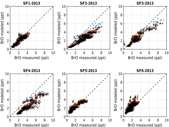
Figure 12.Comparison of measured and modeled BrO for the NASA-ATTREX science flights 1 to 6 in 2013. Black crosses are for model
run no. 583, blue crosses for no. 584, and red crosses for no. 585.
4.4 Comparison of measured and modeled BrO
Measured and modeled BrO are displayed in Figs. 3 to 8 (panel e) together with the modeled Brinorgy partitioning (panel f) and inferred Brinorgy (panel g). Elevated BrO con-centrations are measured within the LS (range 3–9 ppt), and lower BrO concentrations are measured in the TTL (range 0.5–5 ppt), with the smallest BrO concentrations (0.5–1 ppt) occurring near the bottom of the TTL. Overall, this behav-ior is expected from arguments based on the amount and composition of the brominated organic and inorganic source gases, their lifetimes, atmospheric transport, and photochem-istry (e.g., Fueglistaler et al., 2009; Aschmann et al., 2009; Hossaini et al., 2012b; Ashfold et al., 2012; WMO, 2014; Fernandez et al., 2014; Saiz-Lopez and Fernandez, 2016). In particular, for our daytime measurements, it is observed that (a) BrO increases with O3and available Brinorgy and thus altitude and (b) the predicted BrO/Brinorgy ratio decreases towards the bottom of the TTL, where (c) HBr and/or Br atoms may become comparable to BrO, but HOBr does not play a major role in the Brinorgy partitioning. While obser-vation (a) is due to the increased destruction of primarily the short-lived Brorgy species and the efficient reaction of the released Br atoms with increasing altitude and increasing ozone concentrations, observations (b) and (c) are due to re-actions of the Br atoms with CH2O (and less H2O2) into HBr,
which is recycled back by reactions with OH and by variable amounts heterogeneously (depending on the available sur-face of aerosols and cloud particles) to Br atoms, as predicted by Fernandez et al. (2014), and Saiz-Lopez and Fernandez (2016). The predicted minor role of HOBr eventually formed by reactions of OH radicals with heterogeneously produced Br2or by the reaction HO2+BrO and photolytic destruction
of HOBr in the TTL is also noteworthy. While the rate of the former reaction is small due to the short photolytic lifetime of Br2anyway, the rate of the latter reaction is small due to
the small OH concentration in the TTL as compared to pho-tolysis of HOBr during the daytime.
Figure 12 compares measured and modeled BrO. For the majority of all flights (except flight SF4-2014, for which a DOAS retrieval problem exists which causes a constant bias of about 2 ppt in inferred BrO), measured and modeled BrO closely compare for low concentrations (i.e., close to the bottom to the TTL) or are comparable younger air based on measured CH4. For larger BrO concentrations (and older
air), good agreement between the measurement and model is found for SF1-2013, SF5-2013, and SF6-2013 when air of low NO2 concentrations (and predicted low BrONO2
or by considering a detailed scheme for the dehalogenation of sea salt, i.e., bromine activation (e.g., Saiz-Lopez et al., 2004; Fernandez et al., 2014; Schmidt et al., 2016). Adjusting CH2Br2would add 0.4 ppt of Brinorgy or∼0.3 ppt to BrO, thus removing the flight-to-flight scatter in source gas concentra-tions (±0.8 ppt) in Brinorgy . This could for example be done by a detailed back trajectory and source appointment analysis, to which a forthcoming study will be devoted. Likewise, the de-halogenation of sea salt could add another 0.5 ppt to BrO (or about 0.7 ppt of Brinorgy ) in the upper TTL (e.g., Saiz-Lopez et al., 2004; Fernandez et al., 2014; Schmidt et al., 2016).
4.5 Uncertainties in estimating the inorganic bromine partitioning
Another reason for the gap in measured and modeled BrO may come from uncertainties in the kinetic constants used and how they affect the Brinorgy (=Br +2·Br2 + BrO +
BrONO2 + HOBr+HBr +BrCl) partitioning. Our
pho-tochemical modeling, aimed at reproducing measured O3,
NO2, and BrO (see the panels f in Figs. 3 to 8), indicates that
during the daytime HOBr and HBr contribute less than 10 % to Brinorgy . Therefore, we concentrate on the photochemical model errors due to the partitioning primarily among BrO, Br, and BrONO2. In this context, the reactions BrO+NO2 +M→BrONO2+M are the most important, followed by
the photolysis of BrONO2and the reaction Br+O3→BrO +O2.
How uncertainties of the photolytic destruction (J) and three-body formation reaction (k; together referred to as
J / k) of BrONO2 propagate into BrO is tested in model
run no. 584. Here, according to the finding of Kreycy et al. (2013), J / k was increased by a factor 1.7 (+0.4/−0.2) as compared to the Jet Propulsion Laboratory (JPL) recommen-dation (Sander et al., 2011) (see the blue crosses in Fig. 12). Evidently, increasingJ / khelps to close the remaining gap in measured versus modeled BrO, which becomes particularly relevant to reproducing BrO when NO2is large, i.e., in the
subtropical LS.
Furthermore, Sander et al. (2011) estimate the uncertainty in the reaction rate coefficient kBr+O3 at low temperature
(T =190 K) to be±40 % (see comment G31). When only considering the two studies which actually measured rather than extrapolated the reaction rate coefficient into the rel-evant temperature range (T=190–200 K), a smaller uncer-tainty (28 %) is indicated (Michael et al., 1978, and Nicovich et al., 1990). Therefore, in the following, an uncertainty of 28 % for kBr+O3 is assumed. Overall, increasingkBr+O3
(model run no. 585) to the upper limit possible according to the JPL compilation (i.e., by factor of 1.28) changes the measured vs. modeled correlation for BrO very little (see the red crosses in Fig. 12). It does, however, change the Brinorgy partitioning so that [BrO] is always largely preva-lent over [Br] even at the lowest altitudes of the TTL (see,
e.g., panel f in Figs. 3 to 8). Our joint measurement of O3,
NO2, and BrO and the supporting CTM simulations thus
in-dicate [Br]/[BrO]<1 for all probed regimes. Our finding is therefore in contrast to the simulations of Fernandez et al. (2014) and Saiz-Lopez and Fernandez (2016), who suggest that [Br]/[BrO] may become larger than unity in the tropi-cal UT and TTL during the daytime. This conclusion is due mostly to the measured O3concentrations, which are larger
than those modeled in the study of Fernandez et al. (2014) and Saiz-Lopez and Fernandez (2016), and the conclusion is irrespective of what (within the given error bars) is assumed forkBr+O3.
Gaussian addition of all uncertainties and errors (i.e., the errors of the retrieved BrO concentrations (in Sect. 4.4 of Stutz et al., 2016), the cross section error, and the uncertainty in the modeled [Br]/[BrO] and [BrONO2]/[BrO] ratios)
leads to the Brinorgy error, as indicated in panel f of Figs. 3 to 8.
4.6 Inferred total Brinorgy
Finally, we discuss the inferred Brinorgy (contribution 4) as a function of potential temperature in the LS, UT, and TTL over the eastern Pacific during the 2013 convective season (Fig. 13). Here we discriminate between young-air
[CH4] ≥1790 ppb, mostly found within the tropical UT and
TTL (Fig. 13, left panel), and older-air[CH4] ≤1790 ppb
(Fig. 13, right panel), mostly found in the subtropical lower-most stratosphere. The different histograms in Fig. 13 clearly indicate that Brinorgy increases with increasing potential tem-perature, i.e., from 2.63±1.04 ppt atθ=350–360 K (at the bottom of the TTL) to 4.22±1.37 ppt for θ=390–400 K (just above the cold-point tropopause). The inferred Brinorgy thus brackets the modeled [Brinorgy ]=3.02±1.90 ppt pre-dicted to exist at 17 km in the TTL well (Navarro et al., 2015).
The increase in Brinorgy with increasing potential tempera-tureθand decreasing CH4concentration thus reflects the
de-crease in concentrations of brominated VSLS (contribution 3). The correspondence of decreasing Brorgy with increasing Brinorgy concentrations is also found on a sample-to-sample as well as on a flight-to-flight basis. This correspondence keeps [Bry] almost constant within the TTL during an indi-vidual flight, but [Bry] varies from flight to flight in a range of [Bry]=20.3 ppt to 22.3 ppt (Fig. 14).
Moreover, it appears that the increase in Brinorgy with θ mostly corresponds to a decrease in concentrations of the brominated VSLS if only the same (young) air masses of large CH4 concentrations are probed (Fig. 15). For
Bryinorg (ppt)
0 2.5 5 7.5 10 12.5 15
0 25
50 350K–360K
0 25
50 360K–370K
0 25
50 370K–380K
Number of occurrence
0 25
50 380K–390K
0 25
50 390K–400K
0 25
50 SF1 >400K
SF2 SF3 SF5 SF6
Bryinorg (ppt)
0 2.5 5 7.5 10 12.5 15
0 25
50 350K–360K
0 25
50 360K–370K
0 25
50 370K–380K
Number of occurrence
0 25
50 380K–390K
0 25
50 390K–400K
0 25
50 SF1 >400K
SF2 SF3 SF5 SF6
Figure 13.Histogram of Brinorgy occurrence as a function of potential temperature for [CH4]≥1790 ppb (left panel) and [CH4]≤1790 ppb
(right panel). High [CH4] can be considered as a marker for young air mostly found in the freshly ventilated TTL, while low [CH4] can be considered as a marker for aged air mostly found in the subtropical lowermost stratosphere. The mean and the variance of Brinorgy for young
air (left panel) are for θ=350–360 K, 2.63±1.04 ppt; θ=360–370 K, 3.1±1.28 ppt;θ=370–380 K, 3.43±1.25 ppt;θ=380–390 K, 4.42±1.35 ppt;θ=390–400 K, 5.1±1.57 ppt, andθ≥400 K, 6.74±1.79 ppt. Aged air (right panel): forθ=390–400 K, 4.22±1.37 ppt; andθ≥400 K, 7.67±2.72 ppt.
When extrapolating the data points along lines of constant [VSLS]+[Brinorgy ] bromine (grey dashed lines in Fig. 15) for SF1-2013, SF5-2013, and SF6-2013 to [Brinorgy ]=0 and as-suming no bromine is effectively lost in the troposphere, then the apparent concentrations of brominated VSLS at the sur-face should range between 4 and 8.5 ppt. However, larger concentrations of brominated VSLS (some 10 ppt) are fre-quently measured in the boundary layer of the Pacific (e.g., Yokouchi et al., 1997; Schauffler et al., 1998; Wamsley et al., 1998; Yokouchi et al., 2005; Tegtmeier et al., 2012; Ashfold et al., 2012; Ziska et al., 2013; Sala et al., 2014). Further, bromine released from sea salt also contributes to Brinorgy in the marine boundary layer and may reach the bottom of the TTL in variable amounts (e.g., Saiz-Lopez et al., 2004; Fer-nandez et al., 2014; Schmidt et al., 2016). Therefore, effec-tive loss processes for inorganic bromine, for example by the heterogeneous uptake of inorganic bromine on aerosol and cloud particles, must be active in the atmosphere (e.g., Schmidt et al., 2016).
Next, when subtracting the almost constant contribution of CH3Br and the halons to total stratospheric bromine (14.6 ppt
in 2013) from the range (20.3 to 22.3 ppt) of total Brygiven, a variable contribution from VSLS bromine (contribution 3) and Brinorgy (contribution 4) to total TTL bromine in the range of 5.7 ppt to 7.7 ppt (±1.5 ppt) is calculated (Fig. 15). We note that this range falls well into the range assessed in WMO
(2014) and recently estimated by Navarro et al. (2015) (6 ppt; range=4–9 ppt) for contribution of 3 and 4 to the total strato-spheric Bry. It is, however, somewhat (up to 2 ppt) larger than indicated in earlier work, including our balloon-borne studies (for details, see Sect. 1).
Here one may wonder whether (a) this result is significant, (b) some Brinorgy is actually removed by heterogeneous pro-cesses in the TTL (e.g., Aschmann et al., 2011; Aschmann and Sinnhuber, 2013), or (c) TTL Bry shows some season-ality analogous to the “tape recorder” for H2O (e.g., Levine
et al., 2008; Krüger et al., 2008; Fueglistaler et al., 2009; Schofield et al., 2011; Ploeger et al., 2011).
Bry(ppt)
0 5 10 15 20 25
P
ot
ent
ial
temp
erat
ure
(K
)
350 360 370 380 390 400 410
SF1-2013
Bry(ppt)
0 5 10 15 20 25
P
ot
ent
ial
temp
erat
ure
(K
)
350 360 370 380 390 400 410
SF3-2013
Br y(ppt)
0 5 10 15 20 25
P
ot
ent
ial
temp
erat
ure
(K
)
350 360 370 380 390 400 410
SF5-2013
Br y(ppt)
0 5 10 15 20 25
P
ot
ent
ial
temp
erat
ure
(K
)
350 360 370 380 390 400 410
SF6-2013
Figure 14.Bryas a function of potential temperature (θ) for all dives during the 2013 NASA-ATTREX flights when joint measurements of
Brorgy and Brinorgy are available.
Bryinorg (ppt)
0 2 4 6 8 10
VSLS (ppt)
0 2 4 6 8 10
SF1 SF3 SF5 SF6
Figure 15.Brinorgy as a function of the sum of all brominated VSLS
using the same color code as in Fig. 10. If all Brinorgy resulted from destroyed VSL bromine of the same air mass from near the surface, then all data points should follow individual diagonal lines.
from 0.4 forθ in the range 350 to 360 K to 0.3 forθ=390 to 400 K) with increasingθ, is also noteworthy. This may in-dicate a subsequent flattening-out of the air-mass-to-air-mass variability of Brinorgy in aging air due to the photochemical de-cay of the brominated organic source gases and atmospheric mixing processes.
4.7 Implications for ozone
The ozone budget in the TOMCAT/SLIMCAT simulation has been analyzed based on the rate-limiting steps of the catalytic ozone destruction cycles, according to the concept of John-ston and Podolske (1978). The chemical rates are averaged over the eastern Pacific region (20◦S–20◦N, 170–90◦W) for
the duration of the campaign. Within this domain, the net rate of ozone change varied from a loss of−0.3 ppbv day−1
at the base of the TTL (θ=355 K,p=150 hPa) to a produc-tion of+1.8 ppbv day−1at the top (θ=383 K,p=90 hPa). This increase in O3with height is due to the strong vertical
gradient in the production rate of odd oxygen by O2
(see Appendix Sect. A). The dominant contribution to this is through the cycle involving BrO + HO2 to form HOBr.
Overall, the modeled ozone loss cycles which account for the majority of the destruction in this region are those with the rate-limiting steps of the reaction HO2 + O3 to form
OH+2O2 and the reaction of HO2 +HO2 to form H2O2,
i.e., cycles involving HOx species. Therefore, increases in the bromine loading of the TTL caused by possible or ex-pected increases have the potential to deplete ozone in a re-gion where ozone changes have the largest impact on radia-tive forcing (Riese et al., 2012).
Quantifying the radiative impact of the O3 changes
de-scribed above is the beyond the scope of this study. How-ever, we can note that (i) recent work has highlighted the effi-ciency of brominated VSLSs at influencing climate (through changed O3), owing to their efficient breakdown in the UTLS
(Hossaini et al., 2015), and (ii) a significant increase in Bryin this region (from VSLS or other sources) could be important for future climate forcing. The latter could conceivably occur given suggested climate-induced changes to (1) tropospheric transport (e.g., Hossaini et al., 2012b), (2) changes in OH, affecting VSLS lifetimes (Schäfer et al., 2016), (3) and/or an elevated bromine loading in the UT-LS and TTL due to the expected increase in VSLS emissions from the rapidly grow-ing aquaculture industry (WMO, 2014).
5 Conclusions
The subtropical lowermost stratosphere, upper troposphere, and tropopause layer of the eastern Pacific are probed for in-organic bromine during the convective season (February and March 2013). The measurements of CH4, O3, NO2, BrO, and
some important organic brominated source gases are inter-compared with TOMCAT/SLIMCAT simulations. After the simulated TOMCAT/SLIMCAT curtains of O3are projected
onto the measured O3concentrations, measured and modeled
CH4agree well. This agreement is not surprising since O3,
and CH4are strongly anticorrelated (see Fig. 9). It thus
pro-vides evidence that the relevant dynamical processes are rep-resented well in the TOMCAT/SLIMCAT simulations. When the simulated curtains of NO2 are adjusted with the same
parameters as inferred above, excellent agreement is again found between measured and modeled NO2, thus
provid-ing further confidence in our measurement technique, in the modeled NOyphotochemistry, and in our overall approach.
The measured and modeled TTL concentrations of CH2Br2 and CHBr3 are found to compare
reason-ably well to the surface concentrations and atmo-spheric lifetimes of both species adopted in the model ([CHBr3]=1.4 ppt, [CH2Br2]=1 ppt at the surface).
Fur-ther, the contribution to bromine in the LS, UT, and TTL by some other VSLS chloro-bromo-hydrocabrons (6
[CHClBr2,CHCl2Br,CH2ClBr,etc.]) is accounted for by
as-suming a constant surface concentration of 1 ppt in the
model. Flight-to-flight total organic bromine inferred from these VSLS species is found to vary by±1 ppt in the TTL over the eastern Pacific in early 2013, which clearly indicates different origins and possibly atmospheric processing of the investigated air masses.
The measured BrO concentrations range between 3 and 9 ppt in the subtropical LS. In the TTL they range be-tween 0.5±0.5 ppt at the bottom of the TTL and about 5 ppt at θ=400 K, in overall good agreement with the model simulations and the expectation based on the decay of the brominated source gases and atmospheric transport. In the TTL, the inferred Brinorgy is found to increase from a mean of 2.63±1.04 ppt forθin the range of 350–360 K to 5.11±1.57 ppt forθ=390–400 K, whereas in the subtropi-cal LS it reaches 7.66±2.95 ppt forθs in the range of 390– 400 K. The non-negligible Brinorgy found for the lowest alti-tudes of the TTL, i.e., 2.63±1.04 ppt with a range from 0.5 to 5.25 ppt (or close to 0 % up to 25 % of all TTL bromine) is also remarkable. This may indicate a sizable but rather vari-able influx of inorganic bromine into the TTL, largely de-pending on the air mass history, i.e., source region, and at-mospheric transport and processing.
Our findings on LS and TTL Brinorgy are in broad agree-ment with past experiagree-mental and theoretical studies on the processes and the amount of bromine injected by source gas and product gases into the TTL and eventually into the ex-tratropical lowermost stratosphere (Ko et al., 1997; Schauf-fler et al., 1998; Wamsley et al., 1998; Dvortsov et al., 1999; Pfeilsticker et al., 2000; Montzka et al., 2003; Salaw-itch, 2006; Sinnhuber and Folkins, 2006; Hendrick et al., 2007; Laube et al., 2008; Dorf et al., 2006b, 2008; Sinnhu-ber et al., 2009; Salawitch et al., 2010; Schofield et al., 2011; Aschmann et al., 2011; Hossaini et al., 2012b; Ashfold et al., 2012; Hossaini et al., 2012a; Aschmann and Sinnhu-ber, 2013; Sala et al., 2014; Wang et al., 2015; Liang et al., 2014; WMO, 2014; Navarro et al., 2015, and many others). Our study, however, sets tighter limits than previous ones ex-isting on the amount of Brinorgy and Br
org
y , the influx of bromi-nated source and product gases, and the photochemistry of bromine in the TTL and LS.
In particular, our study (re-)emphasizes that (a) variable amounts of VSLS bromine and (b) non-negligible amounts of Brinorgy are also transported into the TTL. While process (a) may strongly depend on the source region and season (Hossaini et al., 2016), process (b) may depend on the ef-ficiency of heterogeneous processing and the removal of some Brinorgy by atmospheric (ice) clouds and aerosols (e.g., Aschmann et al., 2011; Aschmann and Sinnhuber, 2013). Therefore, it is not surprising that TTL Bryis rather variable (i.e., 20.3 to 22.3 ppt) in the season studied.
![Figure 13. Histogram of Br inorg y occurrence as a function of potential temperature for [CH 4 ] ≥ 1790 ppb (left panel) and [CH 4 ] ≤ 1790 ppb (right panel)](https://thumb-eu.123doks.com/thumbv2/123dok_br/18202265.333635/16.918.150.767.97.463/figure-histogram-occurrence-function-potential-temperature-panel-panel.webp)

