www.nonlin-processes-geophys.net/23/419/2016/ doi:10.5194/npg-23-419-2016
© Author(s) 2016. CC Attribution 3.0 License.
Conditions for the occurrence of seismic sequences in a fault system
Michele Dragoni and Emanuele Lorenzano
Alma Mater Studiorum Università di Bologna Dipartimento di Fisica e Astronomia, Viale Carlo Berti Pichat 8, 40127 Bologna, Italy
Correspondence to:Michele Dragoni ([email protected]) and Emanuele Lorenzano ([email protected]) Received: 22 February 2016 – Published in Nonlin. Processes Geophys. Discuss.: 25 February 2016
Revised: 29 September 2016 – Accepted: 28 October 2016 – Published: 16 November 2016
Abstract.We consider a fault system producing a sequence of seismic events of similar magnitudes. If the system is made up ofnfaults, there aren!possible sequences, differing from each other for the order of fault activation. Therefore the order of events in a sequence can be expressed as a per-mutation of the firstnintegers. We investigate the conditions for the occurrence of a seismic sequence and how the order of events is related to the initial stress state of the fault sys-tem. To this aim, we considerncoplanar faults placed in an elastic half-space and subject to a constant and uniform strain rate by tectonic motions. We describe the state of the system by n variables that are the Coulomb stresses of the faults. If we order the faults according to the magnitude of their Coulomb stresses, a permutation of the firstn integers can be associated with each state of the system. This permutation changes whenever a fault produces a seismic event, so that the evolution of the system can be described as a sequence of permutations. A crucial role is played by the differences between Coulomb stresses of the faults. The order of events implicit in the initial state is modified due to changes in the differences between Coulomb stresses and to different stress drops of the events. We find that the order of events is deter-mined by the initial stress state, the stress drops and the stress transfers associated with each event. Therefore the model al-lows the retrieval of the stress states of a fault system from the observation of the order of fault activation in a seismic sequence. As an example, the model is applied to the 2012 Emilia (Italy) seismic sequence and enlightens the complex interplay between the fault dislocations that produced the ob-served order of events.
1 Introduction
Seismic sequences are a characteristic aspect of seismic phe-nomenology. Recent examples in Italy are the 1997–1998 Umbria–Marche sequence (Morelli et al., 2000; Salvi et al., 2000; Santini et al., 2004) and the 2012 Emilia sequence (Scognamiglio et al., 2012; Castro et al., 2013; Pezzo et al., 2013). We call “seismic sequence” a series of earthquakes generated by sources located in a relatively small region (of the order of 100 km) and occurring in a time interval (of the order of a few months) much shorter than the intervals dur-ing which the system is at rest. The interval elapsdur-ing between two seismic sequences in the same region is of the order of several decades at least. We do not include in this def-inition aftershock sequences following a greater event that may have similar features but are strongly conditioned by the main shock.
Sequences are originated by fault systems that produce similar earthquakes as to mechanism and magnitude. A se-quence is typically made up of a small number (<10) of larger events having a medium magnitude, in general be-tween 5 and 6, plus a greater number of smaller events. We take into account the larger events, neglecting the smaller ones.
x
1
r12 r23
2 3 •• • n
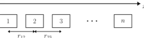
Figure 1.Sketch of the model withncoplanar faults. Thexaxis is the strike direction. Distancesrijbetween theith andjth faults are
computed from the fault centres.
interval, hence reducing the duration of the sequence (e.g. Tallarico et al., 2005).
In the present paper, we consider a model of a fault sys-tem and investigate the conditions under which the syssys-tem may originate seismic sequences with the characteristics de-scribed above. In particular, we ask the following questions.
1. Which are the stress conditions under which a sequence may take place?
2. What determines the order of seismic events in the se-quence?
3. What makes the order of events change from one se-quence to the following one?
4. Is the observed order of events informative about the state of stress before and after the sequence?
The model is applied to the 2012 Emilia (Italy) seismic se-quence that was made up of seven major events with similar focal mechanisms and with magnitudes between 5 and 6, oc-curring in a time interval of 15 days.
2 The model
We consider a system made up ofnplane faults that we as-sume to be coplanar and lined up, with the same strike and dip angles (Fig. 1). The fault system is placed in an elas-tic half-space with Lamé constants λ andµ. We introduce a coordinate system (x,y,z) such that the x axis coincides with fault strike,y is the horizontal direction perpendicular to strike andzis depth. Letδbe the dip angle of the faults.
We number the faults from 1 ton, starting from one end of the system. LetAi be the area of theith fault andrij be the distance between the centres of theith andjth faults. We introduce the following assumptions:
1. the fault system is subject to a strain ratee˙that is con-stant in time and uniform in space;
2. the onset of seismic events is controlled by the average values of tangential traction and static friction on fault surfaces;
3. fault slip is a step function of time and does not produce overshooting;
4. each fault slips once and only once during a sequence;
5. there is no simultaneous slip of two or more faults and a finite time interval elapses between the failures of any two faults;
6. the duration of a sequence is much shorter than the in-terval between two consecutive sequences; and 7. the system is not subject to external stress perturbations. Most of these assumptions are commonly introduced in seis-mic source models. Assumption 1 is reasonable, since by def-inition thenfaults belong to the same seismogenic region, for which the same tectonic mechanism is observed. Assump-tions 2 and 3 are based on the fact that we are not interested in the details of each event, which has a much shorter dura-tion than the duradura-tion of the sequence, but rather in the re-lationship between thenevents. Assumptions 4, 5 and 6 are suggested by the features of the sequences we are describ-ing. Sequences are made up of distinct events, each one as-sociated with the failure of a distinct fault in the system, and there is no observation of reactivation of the same fault dur-ing a sequence. The duration of a sequence is typically sev-eral weeks or a few months, while the interval between two consecutive sequences may even be centuries long (Rovida et al., 2011).
As to assumption 7, it is a fact that the evolution of a fault system can be altered by external perturbations. Any fault system is not isolated, but is surrounded by other faults that may transfer stress to it whenever they slip (e.g. Dragoni and Piombo, 2015). Generally, contributions from external faults may be numerous during an interseismic interval, but they are smaller than contributions from faults belonging to the system, due to greater distances and to different orientations of fault surfaces. Such contributions may also partially cancel each other.
In the case of normal and reverse faults, we assume plane strain, according to the Anderson model (Anderson, 1951; Sibson, 1974; Turcotte and Schubert, 2002). The nonvanish-ing strain components are
eyy= ˙et,
ezz= − λ
λ+2µeyy, (1)
wheree˙ is positive for tensile strain and negative for com-pressive strain. The stress components are
σxx=νσyy,
σyy= 2µ
1−νeyy, (2)
whereνis the Poisson modulus. We introduce the stress rate
˙
σ= 2µ
1−νe.˙ (3)
The rates of normal and tangential traction on the faults are then
˙
σn= −˙ σ
˙
σt = ±˙ σ
2 sin 2δ, (4)
where the upper sign inσt is for normal faults and the lower sign is for reverse faults. In the case of transcurrent faults, we consider simple shear, with strain and stress components
exy= ˙et,
σxy=2µexy. (5)
In this case, we define
˙
σ =2µe˙ (6)
and the rates of normal and tangential traction on the faults are
˙
σn=0, ˙
σt = ˙σ. (7)
Let σi be the average tangential traction applied to the ith fault in the slip direction andτi be the average static friction of theith fault. We define the Coulomb stress (Stein, 1999) of theith fault as
xi=σi−τi,
i=1,2, . . . n. (8)
Since theσiare always positive or zero, thexirange between −τiand zero. Whenxi =0, an earthquake is generated by the ith fault. The rates ofσi andτiare, respectively,
˙
σi = ˙σt,
˙
τi =κσ˙n, (9)
whereκ is the coefficient of static friction. Then the rate of Coulomb stress is
˙
x=kσ,˙ (10)
where
k=sinδ(κsinδ±cosδ) (11) for normal and reverse faults and
k=1 (12)
for transcurrent faults. Then, in the absence of earthquakes, the Coulomb stress of theith fault changes in time as xi(t )=x0i+ ˙xt, (13) wherex0i is the Coulomb stress at an arbitrary timet=0.
Due to the presence of friction, the set of n faults is a nonlinear dynamical system. The Coulomb stresses xi can be considered as the components of ann-dimensional vector
x(t )describing the state of the system as a function of time.
The possible states of the system belong to ann-dimensional parallelepipedS, defined by thendisequalities
−τi≤xi≤0. (14)
According to assumption 5, all the components ofxare
dif-ferent from each other. Therefore one (and only one) com-ponent will vanish first, generating the first event in the se-quence. Whenever an earthquake occurs, the fault dislocation produces a static stress field that is transferred to the system and modifies the Coulomb stress of all faults, producing a sudden change inx.
In general, the change in Coulomb stress on thejth fault due to the failure of theith fault can be written as
1xij(t )=1σijH (t )+1σij′(t ), (15) where1σijis the coseismic change in tangential traction,H is the Heaviside function and1σij′ is the change in traction due to time-dependent processes, including pore fluid diffu-sion, after-slip and viscoelastic relaxation. Since we have as-sumed that faults are coplanar, there are no changes in normal stress on the fault plane.
The traction1σij could be calculated from the formulae for a rectangular dislocation in an elastic half-space collected by Okada (1992). However, ifrij>1.5√Ai, the traction of a finite dislocation source is virtually indistinguishable from that of a point-like double-couple source in an unbounded medium (Love, 1944) and the latter simpler formula can be used (Appendix A).
A Poisson solid (λ=µ) is considered. Accordingly, ifmi is the seismic moment of theith fault, we have
1σij= 5mi 12π rij3,
i6=j (16)
in the case of a strike-slip mechanism and 1σij=
mi
6π rij3,
i6=j (17)
in the case of a dip-slip mechanism. As to the stress change of theith fault, it is
1σii= −1σi, (18)
where1σi is the static stress drop that can be estimated from the average slipui and the fault areaAi as
1σi=C µui √
Ai
, (19)
According to discrete fault models (e.g. Dragoni and Pi-ombo, 2015), the stress drop is a fraction
f =2(1−ǫ) (20)
of static friction, where ǫ is the ratio between the average values of dynamic and static frictions that we assume to be the same for all faults.
If the medium is porous and saturated with fluids, the coseismic stress field induces a fluid flow that changes the stress field in turn (e.g. Wang, 2000; Piombo et al., 2005). As shown in Appendix B, the effect of fluid diffusion is at least 1 order of magnitude smaller than coseismic stress transfer: for the sake of simplicity, we do not consider it in the following. However, in some cases pore fluid diffusion may have a role in the evolution of a seismic sequence (e.g. Convertito et al., 2013).
As to after-slip and viscoelastic relaxation, the events we are considering are relatively small, and it is assumed that they do not produce appreciable after-slip or impose consid-erable stress on deeper ductile regions that may relax it af-terwards. Viscoelastic relaxation of lithospheric rocks may change the stress distribution in the long term as a conse-quence of larger earthquakes (e.g. Dragoni and Lorenzano, 2015).
3 Evolution of the system
Lettk be the occurrence times of the events in the sequence (k=1,2, . . . n), so that the durations of the interseismic in-tervals are
1tk=tk+1−tk,
k=1,2, . . . n−1. (21)
Then the initial state is x(t1−). If the first event is due to
the failure of thei1th fault,xhas a sudden change and itsk
component becomes
xk(t1+)=xk(t1−)+1xi1k. (22) Afterwards, x changes continuously in time, as a
conse-quence of tectonic loading, according to
xk(t )=xk(t1+)+ ˙x(t−t1). (23)
Att=t2, the second event takes place, due to the failure of
thei2th fault, so thatxhas another sudden change, and so on.
At the end of the sequence, the state is
xk(tn+)=xk(tn−)+1xink (24)
that can be written as xk(tn+)=xk(t1−)+ ˙x 1t+
n
X
j=1
1xj k (25)
where
1t= n−1 X
k=1
1tk=tn−t1 (26)
is the duration of the sequence that can be written as
1t= −xin(t1−) ˙
x − 1
˙
x n
X
j=1
1xijin,
ij 6=in. (27)
In Eq. (25) the difference between the final and initial states is made up of two terms: the first one is tectonic loading dur-ing the time interval1t; the second one is the effect of earth-quakes. The latter term has the effect of concentrating in a shorter time interval a series of events that otherwise would be farther in time. The shortening in duration is obtained by calculating how much the instanttnof the last event is antici-pated. The decrease intnis due to the sum of the stresses that are transferred to theinth fault from the othern−1 faults. From Eq. (27), the duration of the sequence in the absence of interaction is
1t′=1t+1
˙
x n
X
j=1
1xijin,
ij6=in. (28)
The interseismic intervals in Eq. (21) can be calculated as 1tk= −
xik+1(tk+)
˙
x ,
k=1,2, . . . n−1. (29)
During the interseismic intervals, the representative pointx
moves along a line defined by the parametric Eq. (13) that is parallel to the line
x1=x2=. . .=xn. (30) Thanks to a rotationR, the coordinate system(x1, . . . xn)can be changed into a system(ξ1, . . . ξn)such that theξnaxis co-incides with line (Eq. 30). Hence the evolution of the system can be more easily represented in the (n−1)-dimensional hyperplaneξn=0. An example will be shown in Sect. 7 for n=3.
4 Retrieval of the initial and final states
On the basis of the model, if we observe a seismic sequence, we can retrieve the state vectorx(t )at any time during the
se-quence. In particular, we can calculate the state of the system at the beginning and at the end of the sequence.
times of the events. From the knowledge of the fault geom-etry and of the seismic moments, we can calculate the stress transfer matrix1xij. If we know the strain ratee˙from geode-tic measurements, we can calculate the stress rate x˙ from Eq. (10).
Consider the generic fault ik that has produced the kth event in the sequence. It is easy to see that the Coulomb stress of faultikat the beginning of the sequence is
xik(t1−)= − ˙x (tk−t1)−
k−1 X
j=1
1xijik. (31)
Apart from the signs, the first term in the rhs is the stress ac-cumulated on the fault from the beginning of the sequence up to instanttkand the second term is the sum of stress trans-fers that faultik has received from faultsi1,i2, . . .ik−1that
slipped before it. Hence, apart from the sign, the rhs is the total stress accumulated on faultiksince the beginning of the sequence. This stress must cancel the initial Coulomb stress xik(t1−): hence the initial Coulomb stress must be the
oppo-site of the accumulated stress.
As to the final state of faultik, it is given by Eq. (25). If we replacexik(t1−)in Eq. (25) with its expression (Eq. 31),
we obtain
xik(tn+)= ˙x (tn−tk)+
n
X
j=k
1xijik. (32)
Since the Coulomb stress of fault ik was equal to zero at t=tk−, the final stress is equal to the tectonic stress accu-mulated in the time interval fromtk totnplus the stress drop associated with the failure of faultikand the stress transfers of the faultsik+1,ik+2, . . . inthat have slipped after faultik. Hence the initial Coulomb stress of faultik depends only on what happened before the instant tk, while the final Coulomb stress depends only on what happened after tk. However, the retrieval of the complete state vector requires the knowledge of the entire sequence. In Sect. 8, we shall retrieve the initial and final states of a fault system in a real case.
The degree of heterogeneity of thexi can be expressed by their standard deviation
s= "
1 n
n
X
i=1
(xi− ¯x)2
#1/2
, (33)
where
¯
x=1 n
n
X
i=1
xi. (34)
A relevant point for the subsequent evolution is whether the differences between thexichange during a sequence. We de-fine
dij(t )=xi(t )−xj(t ). (35)
Thedij form an antisymmetric matrix havingn(n−1) non-vanishing components that are related by(n−1)2equations. Thereforedij is known if we know onlyn−1 components, for example thed1j withj=2,3, . . . n. Thanks to Eq. (32), we obtain
dij(tn+)−dij(t1−)=
n
X
k=1
(1xki−1xkj), (36)
where the rhs is different from zero because the sum of stress transfers received by a fault during the sequence is in general different from that received by the other faults. In particular, faults located at the centre of the system receive a greater total stress than faults located at the ends, if the events have similar magnitudes. For instance, ifn=3, fault 2 receives a greater stress transfer than faults 1 and 3.
5 The order of events
Since the componentsxiof the state vector are always differ-ent from each other, they can be ordered according to their magnitudes. Then, at any instantt of time, the setX of the xi(t )is a well-ordered set. This order controls the order of events in the seismic sequence.
LetNnbe the set of the firstnnatural numbers. With each statexof the system we can associate a permutationαofNn,
expressing the order of faults in relation to the value of their Coulomb stress:
α=
1 2 . . . n i1 i2 . . . in
, (37)
so that
xi1=maxX, (38)
xik=max(X− {xi1, xi2, . . . xik−1}), (39) withk=2,3, . . . n. Hence the parallelepiped S can be di-vided into a numbern! of subsetsSj corresponding to the n!permutations ofNn. During the interseismic intervals, the permutationαj associated with the system does not change, because all thexi increase with the same rate, according to Eq. (13). Thereforexremains in the same subsetSj.
How-ever, when an event occurs,x switches to a different subset
Sk, characterized by a permutationαk.
Suppose that, before the sequence, the permutation asso-ciated with the system is
α0=
1 2 . . . n i1 i2 . . . in
, (40)
implying that the first event is the failure of thei1th fault.
This event changes the magnitudes of all Coulomb stresses, so that the new state of the system is associated with a differ-ent permutation
α1=
1 2 . . . n j1 j2 . . . jn
implying that the second event is the failure of thej1th fault,
and so on. After the(n−1)th event, the permutation is αn−1=
1 2 . . . n k1 k2 . . . kn
, (42)
implying that the last event is the failure of the k1th fault.
Therefore the order of events in the sequence can be ex-pressed as a permutation
α∗=
1 2 . . . n i1 j1 . . . k1
. (43)
As to the order of events, the number of possible sequences in a system made up ofnfaults is equal ton!. Since every fault may slip only once in a sequence (assumption 4), there aren! alternatives for the initial permutation α0, but only(n−1)!
forα1and(n−k)!for the generic permutationαk. If the permutation after thenth event is
αn=
1 2 . . . n i j . . . k
, (44)
the duration of the interseismic interval preceding the next sequence is
1T = −xi(tn+)
˙
x (45)
and the sequence will start with the failure of theith fault. In order to find out the relationship between the initial permuta-tionα0and the order of events given byα∗, it is necessary to
examine which are the orders of magnitude of the quantities controlling the evolution of the system.
6 Discussion
The evolution of the system is controlled by the stress rate
˙
σ and by the stress transfer matrix1xij. We calculate the typical values of these quantities for seismic sequences.
For many seismogenic regions, typical strain rates are of the order of 10−15 to 10−14s−1. With µ=30 GPa and ν=0.25, Eq. (3) and Eq. (6) yield stress rates| ˙σ|of the or-der of 2 kPa a−1for the lower value and of 20 kPa a−1for the higher value of the strain rate. Calculation of 1xij requires the knowledge of the seismic moments associated with each fault, of the fault areas and of the distances between them. A typical seismic moment of an event in the sequence can be calculated by assuming an area Ai=100 km2and an aver-age slipui=0.5 m; hence,mi ≃1018N m. With these val-ues, Eq. (19) yields a stress drop1σi≃1 MPa. This value corresponds to the stress that is accumulated in a time in-tervalt0=500 a at a rate of 2 kPa a−1or t0=50 a at a rate
of 20 kPa a−1. From Eq. (20) with a typical value ǫ=0.7 (Scholz, 1990), we obtain1σi=0.6τi.
As to the distance between the centres of two neighbour-ing faults, we may roughly assume thatr=2√Ai =20 km.
Then, according to Eqs. (16) and (17), the stress1σij trans-ferred from a fault to its first neighbours is of the order of 10 kPa, so that the maximum value of1σij (i6=j) is of the order of one-hundredth of a stress drop. It must be noted that a greater value ofmi does not entail a proportionally greater value of1σij, because it implies a greater fault area and a greater distance between faults.
An obvious effect of fault interaction is the shortening of time intervals between seismic events: for neighbouring faults, the gained time1σij/| ˙σ|ranges from 5 to 0.5 a ac-cording to the value ofσ˙. Hence the maximum stress trans-ferred by one event is equivalent to several months or several years of tectonic loading.
The magnitude of the differences dij between Coulomb stresses is critical for the occurrence of a sequence. A lower limit fordijis set by the magnitude of transferred stress1σij (i6=j). Ifdijis smaller than1σij, the failure of theith fault would immediately produce the failure of thejth fault, in contrast to assumption 5. Hence a condition for having a se-quence ofndistinct events isdij> 1σijat any time.
An upper limit fordij is set by the observed durations of seismic sequences. Thedij must be small enough that a se-quence is completed within a few months, if we take into account the effect of stress transfer between faults. Hence we may assume as an upper limit fordij the stress change
˙
x δt that tectonic loading produces in a timeδt ≪1T (as-sumption 6) plus the sum of transferred stresses1xij(i6=j). A greater value forδt (several decades) can be assumed for lower stress rates, a smaller value (several years) for higher stress rates.
With this premise, we consider how the orderα∗of events in a sequence is determined. The quantities determiningα∗ are the initial stress state of the fault system, the stress drops and the stress transfers associated with each event.
The simplest case is when the stress drops are about equal to each other and thedij are always greater than the trans-ferred stresses1xij (i6=j). If these conditions are fulfilled, the only effect of thekth event is to shift the labelik to the last position in the permutationαk, while the stress transfers 1xikjdo not change the relative positions of the other labels.
So we can associate with each event a permutation η=
i1 i2 . . . in i2 i3 . . . i1
(46) such that
αk=ηαk−1. (47)
It follows that the order of events is given by the initial per-mutation, i.e.α∗=α0. The final permutationαnis also equal toα0, but this does not imply the repetition of the orderα∗
in the following sequence. According to Eq. (36), the new sequence will start with different values ofdij that may pro-duce a different order of events.
Apart from the case just described, the order implied byα0
the same order of magnitude as the1xij(i6=j). In addition, if an event j has a stress drop that is considerably greater than the others, the labelij will permanently occupy the last position in the permutation, thus altering the initial order. It follows that the order of events is different from the initial order of stresses, i.e. α∗6=α0. The final permutationαn is also different fromα0.
7 An example: the casen=3
As an example, we consider a system made up of three faults with a strike-slip mechanism. This case is considered be-cause it can be illustrated graphically, owing to the small number of variables involved. Cases with n >3 would re-quire higher-dimensional spaces. The graphical representa-tion allows a better understanding of the evolurepresenta-tion of the state of the fault system during a seismic sequence.
For the sake of simplicity, we suppose that the faults are equal to each other, with distances r12=r23=20 km
be-tween their centres. With a strain rate e˙=10−14s−1, the stress rate calculated from Eq. (6) is σ˙ ≃19 kPa a−1. For the sake of simplicity, we suppose that the faults have the same static frictionτ =1 MPa and produce events with the same seismic moment m0=1018Nm. The stress transfer
matrix Eq. (15) is symmetric, with nondiagonal components 1x12≃17 kPa and1x13≃2 kPa. With a typical valueǫ=
0.7, Eq. (20) yields stress drops1xi=600 kPa.
We consider coordinatesxi/τ. The parallelepiped S is a cube with unit edge, defined by the disequalities
−1≤xi/τ ≤0 (48)
and can be divided into six subsetsSj corresponding to the six permutations ofN3. During the interseismic intervals, the
representative pointx(t )of the system draws an orbit parallel
to the line
x1=x2=x3. (49)
An event occurs whenever the point reaches one of the coor-dinate planes.
As anticipated in Sect. 3, we can rotate the coordinate sys-tem so that theξ3axis coincides with line (Eq. 49). It is easy
to see that
R=
b −c −a
−c b −a
a a a
, (50)
where a=√1
3, b=1+a
2 , c=1−a
2 . (51)
The projection ofSon the planeξ3=0 is a regular hexagon
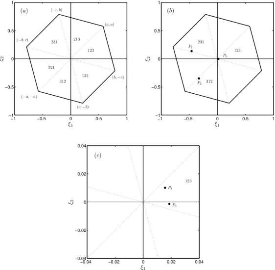
H with sidea(Fig. 2a). It is divided into six equilateral tri-anglesHk that are the projections of the subsetsSk. We can follow the evolution of the system by looking at the projec-tionP of the representative point onH. During the interseis-mic intervals,P does not change, because the representative point moves on a line perpendicular toH, and is close to the origin, because thedij are much smaller thanτ. Whenever an event takes place,P moves to a different subset ofH.
Suppose that, at a certain instantt0of the interseismic
in-terval preceding a sequence, the state of the system is
x0=x(t0)=(x01, x02, x03) (52)
withx01> x02> x03. The associated permutation is then
α0=
1 2 3
1 2 3
(53) and the representative pointP0belongs to the subset of H
labelled with 123 in Fig. 2b. We choose the vectorx0in
or-der that the sequence is made up of three distinct events, oc-curring in the order given byα0. Thend12 andd13 must be
positive, withd12< d13. According to the discussion in the
previous section,
1x12< d12< d13< 1x13+1x23+ ˙σ δt, (54)
where we assume δt=1 a, so that σ δt˙ ≃19 kPa. Then 17 kPa< d12< d13<38 kPa and we choose d12=20 kPa
andd13=25 kPa. At the beginning of the sequence, the state
is
x(t1−)=(0, d21, d31). (55)
The mean is x¯= −15 kPa, with a standard deviation s= 10 kPa. The state immediately after the first event is
x(t1+)=(1x11, d21+1x12, d31+1x13). (56)
According to Eq. (47), the associated permutation isα1=
ηα0with
η=
1 2 3
2 3 1
(57) and the representative pointP1belongs to the subset of H
labelled with 231 in Fig. 2b. From Eq. (29), the time interval between the first and second events is1t1=66 d. At the end
of this interval, the state is
x(t2−)=(x1(t1+)+ ˙σ 1t1,0, x3(t1+)+ ˙σ 1t1) (58)
and the second event takes place. The state becomes
x(t2+)=(x1(t2−)+1x21, 1x22, x3(t2−)+1x23). (59)
The associated permutation isα2=ηα1and the
−1 −0.5 0 0.5 1 −1
−0.5 0 0.5 1
ξ1 ξ2
(a)
123 213 231
321
312 132
(a, a)
(−c, b)
(−b, c)
(−a,−a)
(c,−b)
(b,−c)
−1 −0.5 0 0.5 1
−1 −0.5 0 0.5 1
ξ1 ξ2
(b)
P0
P1
P2
123 231
312
−0.04 −0.02 0 0.02 0.04
−0.04 −0.02 0 0.02 0.04
ξ1 ξ2
(c)
P0
P3
123
Figure 2.Evolution of a system made up of three faults (n=3), represented in the state space:(a)the hexagonH, defined in Sect. 7, with its subsets labelled by the associated permutations;(b)states of the system during a seismic sequence:P0is the initial state;Pi (i=1,2,3)
is the state after theith event of the sequence;(c)magnification ofH showing the initial and final statesP0andP3.
in Fig. 2b. The time interval between the second and third events is1t2=56 d. Att=t3−the state is
x(t3−)=(x1(t2+)+ ˙σ 1t2, x2(t2+)+ ˙σ 1t2,0). (60)
The third event takes place and the state becomes
x(t3+)=(x1(t3−)+1x31, x2(t3−)+1x32, 1x33) (61)
withα3=ηα2, which coincides withα0. The representative
point P3 belongs to the subset of H labelled with 123 in
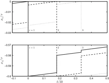
Fig. 2c. According to Eq. (26), the duration of the sequence is 1t=122 d. In the absence of interaction, the duration would have been 1t′=482 d from Eq. (28). The evolution of the three components in time is shown in Fig. 3.
The final state is very different from the initial one, with a value of x¯ that is about 40 times greater, while s has not changed. The differences between components ared12=
5 kPa andd13=25 kPa, so thatx2 has become closer tox1
and farther from x3. In fact, the state no longer fulfills the
conditiond12> 1x12, entailing that, when the next sequence
occurs, the stress1x12 transferred to fault 2 by the slip of
fault 1 will induce the immediate failure of fault 2.
According to Eq. (45), the duration of the time interval be-fore the next sequence is1T ≃30 a. Even though the order of events in this sequence is the same as in the previous one, the durations of the intervals1tkare different. Moreover, the stress distribution is altered in such a way thatα36=α0,
en-tailing that even the order of events will be different in the following sequence.
−0.03 −0.02 −0.01 0
xi
/
τ
i= 1 2 3
−0.1 0 0.1 0.2 0.3 0.4 0.5
−0.6 −0.59 −0.58 −0.57
t/δt
xi
/
τ
i= 1 2 3
Figure 3.Evolution of a system made up of three faults (n=3): components of the state vectorx as functions of time during the seismic sequence shown in Fig. 2 (τ=1 MPa,δt=1 a). The steps labelled byi=1, 2 and 3 correspond to the occurrence of the events in the sequence.
Figure 4.Geographic location of the 2012 Emilia seismic sequence (Italy). Stars indicate the epicentres; numbers indicate the order of fault activation.
8 The 2012 Emilia sequence
We consider the 2012 Emilia (Italy) seismic sequence that was made up of seven events with magnitudes between 5 and 6 (Pezzo et al., 2013). They occurred in the period between 20 May and 3 June 2012, and can be ascribed to a fault sys-tem approximately lined up in the west–east direction, with a total length of about 50 km. The faults are all of thrust type and with shallow hypocentres between 5 and 10 km in depth (Fig. 4).
The Emilia sequence has been studied in detail by several authors, who determined the locations and seismic moments of the events (Scognamiglio et al., 2012), the source
func-1 2 3 4 5 6 7
Event number 0
20 40 60 80 100
mi
(
"
1
0
1
6N
m
)
5 6 7 4 3 2 1
Fault number
Figure 5.Seismic momentsmiof the events in the 2012 Emilia
se-quence. The upper scale indicates the fault number, the lower scale the order of activation. The two strings of numbers yield the permu-tationα∗in Eq. (62).
tions and seismic spectra (Castro et al., 2013) and the coseis-mic deformation (Pezzo et al., 2013). Convertito et al. (2013) suggested that dynamic triggering caused by seismic waves might be the primary factor to explain the evolution of the Emilia sequence, in addition to the variation in permeability and pore-pressure effects due to a massive presence of fluids in the Po Plain basin.
As stated in Sect. 2, we neglect the effect of pore fluid diffusion, on the basis of considerations in Appendix B, as well as the possible effect of seismic waves. Our aim is not to simulate the Emilia sequence in detail, but to use it as an example of a complex sequence for which the present model can afford the retrieval of the initial and final stress states. If further effects are relevant and are introduced in the cal-culations, they may alter the sequence of permutations and yield a different final permutation. However, they would not change the general conclusions of the paper.
According to the model, we approximate the real fault sys-tem with a set ofn=7 faults having the same strike and dip angles and the same average depth. If we number the faults from west to east, the order of events is given by
α∗=
1 2 3 4 5 6 7
5 6 7 4 3 2 1
. (62)
Therefore, fault slip started about the middle of the system and propagated eastward up to the end of the system (5, 6, 7); then it propagated from the middle to the west end (4, 3, 2, 1) (Fig. 5).
⋆ 1 ⋆ 2 ⋆ 3 ⋆ 4 ⋆ 5 ⋆ 6 ⋆ 7 W E
Figure 6.Geometry of the model for the 2012 Emilia seismic se-quence. The rectangles are the projections of faults on a vertical plane. Faults are numbered from west to east. Stars indicate the hypocentres.
1 2 3 4 5 6 7
−0.1 −0.08 −0.06 −0.04 −0.02 0 Fault number xi (M P a) ¯ x ¯
x+s
¯
x−s
(a)
1 2 3 4 5 6 7
−2 −1.5 −1 −0.5 0 Fault number xi (M P a) ¯ x ¯
x+s
¯
x−s
(b)
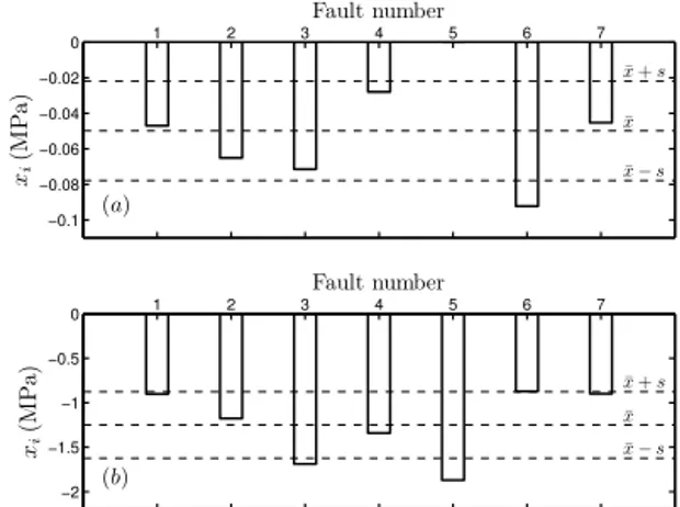
Figure 7.Components of the state vectorxat the beginning(a)and at the end(b)of the 2012 Emilia seismic sequence, as calculated from the model. Faults are numbered from west to east. The mean
¯
xand the standard deviationsare shown.
As to the elastic and frictional properties, we take µ= 30 GPa,ν=0.25 and an effective coefficient of frictionκ= 0.6. The areas and the locations of the faults have been inferred by employing the distances between hypocentres along the strike direction as constraints (Caporali and Os-tini, 2012; Serpelloni et al., 2012). The distances between the centres of the faults arer12=r23=r67=5 km,r34=r56=
8 km, andr45=12 km. The projection of the faults on a
ver-tical plane is shown in Fig. 6.
We treat all sources as pure reverse, dip-slip faults with δ=40◦, an average of the values given by Convertito et al. (2013). The strain rate is e˙= −3×10⁻¹⁵s−1(Caporali and Ostini, 2012). The momentsmiare derived from the mo-ment magnitudes reported in Tramelli et al. (2014), whereas fault slips ui are calculated from mi andAi. The data are shown in Table 1. From Eq. (19) withC=1, the values of stress drops1σi are in the range between 0.9 and 1.9 MPa, consistent with the range evaluated by Castro et al. (2013) from seismic spectra.
From these data we calculate the ratex˙of Coulomb stress and the stress transfer matrix 1xij. From Eq. (10), x˙ ≃ 2 kPa a−1. The initial statex(t1−)and the final statex(t7+)
are shown in Fig. 7. The initial and final permutations are, respectively,
α0=
1 2 3 4 5 6 7
5 4 7 1 2 3 6
, (63)
α7=
1 2 3 4 5 6 7
6 7 1 2 4 3 5
. (64)
The evolution of the system during the sequence shows that Eq. (47) does not hold for any value ofk. Therefore α7 is
different fromα0and they are both different fromα∗. This
is a consequence of the heterogeneous distribution of seis-mic moment in the fault system. In particular, the evolution of stress was conditioned by the first and fourth events, due to the failures of faults 5 and 4, respectively, having greater seismic moments than the average. As a consequence of the greater stress drop, fault 5 permanently occupies the last po-sition in all permutations fromα1toα7. The stress transfers
associated with each event also play a role in determining the evolution of the sequence, contributing to the rearrangement in the permutations. Due to the many stress transfers to fault 6, Eq. (28) yields1t′ ≃ 46 a for the duration of the sequence in the absence of fault interaction, a much longer time than the observed duration1t ≃ 15 d.
Figure 6 shows that, at the beginning of the sequence, the mean Coulomb stress wasx¯ ≃ −0.05 MPa, with a stan-dard deviations≃0.03 MPa, whereas at the end of the se-quencex¯≃ −1.2 MPa ands≃0.4 MPa. Therefore Coulomb stresses are much more spread out after the sequence than before, since the standard deviation is 1 order of magnitude larger.
According to Eq. (64), the faults with the highest values of xi after the sequence are the sixth, seventh and first, show-ing that, in the absence of external perturbations, the next sequence would start in the proximity of one end of the sys-tem, rather than in the middle as the 2012 sequence. Accord-ing to Eq. (45), the next sequence will take place after an interseismic interval1T ≃440 a. This figure appears to be representative of typical recurrence times of moderate-size earthquakes in this area: the largest event before the 2012 sequence was theMw5.5 17 November 1570, Ferrara
earth-quake (Rovida et al., 2011).
9 Conclusions
The aim of this study was to enlighten the conditions allow-ing the occurrence of seismic sequences and the processes controlling the order of events in a sequence. When we ob-serve a sequence, we acknowledge that it is due to a system ofnfaults that fail one after the other. However, we do not know why the faults fail in that particular order. The order must be a consequence of the initial stress state of the fault system and of the mutual interaction between faults.
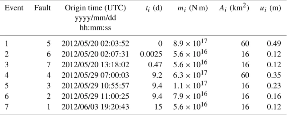
ac-Table 1.Data for the seismic events of the 2012 Emilia sequence. The origin times and the seismic momentsmi are taken from Pezzo et
al. (2013) and Tramelli et al. (2014), respectively. The areasAitake into account the analysis of Caporali and Ostini (2012) and Serpelloni
et al. (2012). Fault slipsuiare calculated frommiandAi. See Fig. 6 for fault numbers.
Event Fault Origin time (UTC) ti(d) mi(N m) Ai (km2) ui(m)
yyyy/mm/dd hh:mm:ss
1 5 2012/05/20 02:03:52 0 8.9×10¹⁷ 60 0.49
2 6 2012/05/20 02:07:31 0.0025 5.6×10¹⁶ 16 0.12
3 7 2012/05/20 13:18:02 0.47 5.6×10¹⁶ 16 0.12
4 4 2012/05/29 07:00:03 9.2 6.3×10¹⁷ 60 0.35
5 3 2012/05/29 10:55:57 9.4 1.1×10¹⁷ 16 0.23
6 2 2012/05/29 11:00:25 9.4 7.9×10¹⁶ 16 0.16
7 1 2012/06/03 19:20:43 15 5.6×10¹⁶ 16 0.12
tivation of faults in the sequence yields information on the state of the fault system before and after the sequence.
The evolution of the fault system during a seismic se-quence can be better understood if we consider the state space. Since a permutation can be associated with each state of the system, the state space can be divided inton!subsets corresponding to then!permutations. The permutation does not change as long as the system is at rest, so that the state remains in the same subset of the state space. Whenever a seismic event takes place, the order of Coulomb stresses is changed and is expressed by a different permutation: an event corresponds to a switch of the state vector to a different sub-set of the state space.
We are now in a position to answer the questions we asked in the Introduction.
1. The occurrence of seismic sequences requires partic-ular stress conditions. A crucial role is played by the differences between the Coulomb stresses of faults. A lower limit for these differences is set by the magni-tude of transferred stresses and an upper limit by the ob-served durations of seismic sequences. This constrains their values in a narrow interval of the order of tens of kPa.
2. The order of events in a sequence is determined by the initial distribution of Coulomb stresses, by the stress drops and by the stress transfers associated with each event. The order of events that is implicit in the initial state is generally modified by the changes in the state vector intervening during the sequence. The dominant contribution to stress changes is given by stress drops that are typically 100 times greater than stress transfers. However, stress transfers have a major role both in an-ticipating the occurrence times of the events and in al-tering the order of events implicit in the initial state. 3. The characteristics of consecutive sequences originated
by a fault system are bound to change. The order implicit in the initial stress distribution is generally
changed during the sequence, because the stress trans-fers between faults have the same order of magnitude as the differences in Coulomb stresses and because one or more events in the sequence may have greater stress drops than the others. In all cases, the state of the system at the end of a sequence is different from the initial one, entailing that the durations of the interseismic intervals between consecutive sequences and between events in a sequence are different.
0 0.5 1 1.5 2 0
0.5 1 1.5 2
(a)
r/L
(
σt
/
µ
)
·
1
0
4
0 0.5 1 1.5 2
0 0.5 1 1.5 2
(b)
r/L
(
σt
/
µ
)
·
1
0
4
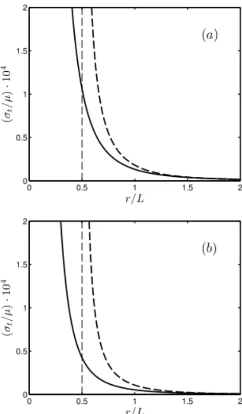
Figure A1.Tangential traction produced by a dislocation in the slip direction on the fault plane in the case of a point-like source in an unbounded medium (solid lines) and a finite source in a half-space (dashed lines):(a)strike-slip;(b)dip-slip.
Appendix A
We consider two different sources: a point-like dislocation (a double couple of forces) in an unbounded elastic medium and a finite square dislocation in an elastic half-space. For both sources, we calculate the tangential tractionσtproduced on the fault plane in the slip direction, as a function of the distance from the source along the strike directionx.
We assume that the elastic medium is a Poisson solid with rigidity µ. The fault lays on the planey=0 and its centre is in the origin of the coordinate system. Let nbe the unit
vector perpendicular to the fault andmbe the unit vector in
the slip direction, so that
n=(0,1,0),
m=(cosθ,0,sinθ ), (A1)
whereθ is the rake angle. The tangential traction in the slip direction is then
σt =σijminj, (A2) whereσij is the stress tensor. We compare the tractions pro-duced by the two sources in two cases: a strike-slip fault (θ=0) and a dip-slip fault (θ=π/2). In the two cases, we haveσt=σxy andσt =σyz, respectively. Letm0be the
scalar seismic moment of the dislocation.
a. In the case of a point-like source, the moment tensor of the equivalent double couple has nonvanishing compo-nents
Mxy= −m0cosθ,
Myz= −m0sinθ. (A3)
The displacement is
ui=Mj kGij,k, (A4) where
Gij= 1 8π µ
r,kkδij− 2 3r,ij
(A5)
is the Somigliana tensor and r=
q
x2+y2+z2. (A6)
In the caseθ=0, we have
σt=µ(ux,y+uy,x). (A7) Settingy=0 andz=0, we obtain
σt(r)= 5m0
12π r3, (A8)
wherer= |x|. In the caseθ=π/2, we have
σt=µ(uy,z+uz,y). (A9) Setting againy=0 andz=0, we obtain
σt(r)= m0
6π r3. (A10)
b. The displacement produced by a finite, rectangu-lar source in an elastic half-space was given by Okada (1992). We consider a square source with side Land centre at depthL. The dip angle isδ=π/4. The analytical expressions ofσt(r)are too complicated to be reported here and we only show their graphs.
0 1 2 3 4 5 −1.5
−1 −0.5 0 0.5 1 1.5
f
(
t
)
t/τ
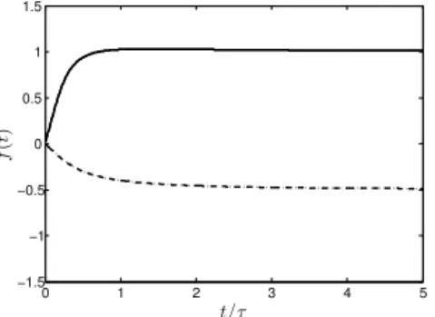
Figure B1.Functionf (t )in the case of strike-slip (solid line) and dip-slip (dashed line). Time is in units of the characteristic diffusion timeτ.
Appendix B
Solutions for a point-like dislocation in a homogeneous and isotropic poroelastic medium are given by Cheng and De-tournay (1998) and Carvalho and Curran (1998). The stress field is made up of a constant term (the coseismic stress) plus a time-dependent term associated with fluid diffusion. We in-troduce a dimensionless variable
ξ(t )= rij
2√ct, (B1)
wherecis the hydraulic diffusivity and a coefficient a= νu−ν
(1−ν)(1−νu)
, (B2)
where νu is the undrained Poisson modulus. When the ith fault slips with momentmi, the additional tangential traction on thejth fault is
1σij′(t )= ami
2π rij3f (t ) (B3) where
f (t )= −√2 πξ e
−ξ2
+3erfξ ξ2 −
6
√
π e−ξ2
ξ +erfcξ (B4) for strike-slip and
f (t )= −3 4
erfξ ξ2 +
3 2√π
e−ξ2 ξ −
1
2erfcξ (B5)
for dip-slip (Fig. B1). Fort→ ∞, the traction Eq. (B3) ap-proaches an asymptotic value
1σij∞= ami
2π rij3 (B6)
for strike-slip and 1σij∞= − ami
4π rij3 (B7)
for dip-slip. According to the choice of a Poisson solid, we take νu=0.25. For a typical valueν=0.2 under drained conditions (e.g. Rice and Cleary, 1976), it results ina≃0.1. Then the ratio
1σ
∞
ij
/1σij between the asymptotic
Acknowledgements. We are grateful to the editor Ilya Zaliapin and to two anonymous reviewers for constructive comments on the first version of the paper.
Edited by: I. Zaliapin
Reviewed by: two anonymous referees
References
Anderson, E. M.: The Dynamics of Faulting, 2nd ed., Oliver and Boyd, Edinburgh, 206 pp., 1951.
Belardinelli, M. E., Bizzarri, A., and Cocco, M.: Earthquake trig-gering by static and dynamic stress changes, J. Geophys. Res., 108, 2135, doi:10.1029/2002JB001779, 2003.
Caporali, A. and Ostini, L.: Analysis of the displacement of geode-tic stations during the Emilia seismic sequence of May 2012, Ann. Geophys., 55, 4, 767–772, doi:10.4401/ag-6115, 2012. Carvalho, J. L. and Curran, J. H.: Three-dimensional displacement
discontinuity solutions for fluid-saturated porous media, Int. J. Solids Struct., 35, 4887–4893, 1998.
Castro, R. R., Pacor, F., Puglia, R., Ameri, G., Letort, J., Massa, M., and Luzi, L.: The 2012 May 20 and 29, Emilia earthquakes (Northern Italy) and the main aftershocks: S-wave attenuation, acceleration source functions and site effects, Geophys. J. Int., 195, 597–611, doi:10.1093/gji/ggt245, 2013.
Cheng, A. H.-D. and Detournay, E.: On singular integral equations and fundamental solutions of poroelasticity, Int. J. Solids Struct., 35, 4521–4555, 1998.
Convertito, V., Catalli, F., and Emolo, A.: Combining stress trans-fer and source directivity: the case of the 2012 Emilia seismic sequence, Sci. Rep., 3, 3114, doi:10.1038/srep03114, 2013. Dragoni, M. and Lorenzano, E.: Stress states and moment rates of a
two-asperity fault in the presence of viscoelastic relaxation, Non-lin. Processes Geophys., 22, 349–359, doi:10.5194/npg-22-349-2015, 2015.
Dragoni, M. and Piombo, A.: Effect of stress perturbations on the dynamics of a complex fault, Pure Appl. Geophys., 172, 2571– 2583, doi:10.1007/s00024-015-1046-5, 2015.
Gomberg, J., Beeler, N. M., and Blanpied, M. L.: On rate-state and Coulomb failure models, J. Geophys. Res., 105, 7557–7871, 2000.
Harris, R. A.: Introduction to special section: Stress triggers, stress shadows, and implications for seismic hazard, J. Geophys. Res., 103, 24347–24358, 1998.
Kanamori, H.: Energy budget of earthquakes and seismic efficiency, Earthquake Thermodynamics and Phase Transformations in the Earth’s Interior, Academic Press, 293–305, 2001.
Love, A. E. H.: A Treatise on the Mathematical Theory of Elasticity, 4th edition, Dover Publications, New York, 643 pp., 1944. Morelli, A., Ekström, G., and Olivieri, M.: Source properties of the
1997–1998 Central Italy earthquake sequence from inversion of long-period and broadband seismograms, J. Seismol. 4, 365–375, 2000.
Okada, Y.: Internal deformation due to shear and tensile faults in a half-space, Bull. Seismol. Soc. Am., 82, 1018–1040, 1992. Pezzo, G., Boncori, J. P. M., Tolomei, C., Salvi, S., Atzori, S.,
An-tonioli, A., Trasatti, E., Novali, F., Serpelloni, E., Candela, L., and Giuliani, R.: Coseismic deformation and source modeling of
the May 2012 Emilia (Northern Italy) earthquakes, Seismol. Res. Lett., 84, 645–655, 2013.
Piombo, A., Martinelli, G., and Dragoni, M.: Post-seismic fluid flow and Coulomb stress changes in a poroelastic medium, Geophys. J. Int., 162, 507–515, 2005.
Rice, J. R. and Cleary, M. P.: Some basic stress diffusion solutions for fluid-saturated elastic porous media with compressible con-stituents, Rev. Geophys. Space Phys., 14, 227–241, 1976. Rovida, A., Camassi, R., Gasperini, P., and Stucchi, M. (Eds.):
CPTI11, the 2011 version of the Parametric Catalogue of Ital-ian Earthquakes, Milano, Bologna, available at: http://emidius. mi.ingv.it/CPTI (last access: 11 November 2016), 2011. Salvi, S., Stramondo, S., Cocco, M., Tesauro, M., Hunstad, I.,
Anzidei, M., Briole, P., Baldi, P., Sansosti, E., Fornaio, G., La-nari, R., Doumaz, F., Pesci, A., and Galvani, A.: Modelling co-seismic displacements resulting from SAR interferometry and GPS measurements during the 1997 Umbria-Marche seismic se-quence, J. Seismol., 4, 479–499, 2000.
Santini, S., Baldi, P., Dragoni, M., Piombo, A., Salvi, S., Spada, G., and Stramondo, S.: Montecarlo inversion of DInSAR data for dislocation modeling: Application to the 1997 Umbria-Marche seismic sequence (Central Italy), Pure Appl. Geophys., 161, 817– 838, 2004.
Scholz, C. H.: The Mechanics of Earthquakes and Faulting, Cam-bridge University Press, CamCam-bridge, 439 pp., 1990.
Scognamiglio, L., Margheriti, L., Mele, F. M., Tinti, E., Bono, A., De Gori, P., Lauciani, V., Lucente, F. P., Mandiello, A. G., Marcocci, C., Mazza, S., Pintore, S., and Quintiliani, M.: The 2012 Pianura Padana Emiliana seismic sequence: Locations, moment tensors and magnitudes, Ann. Geophys., 55, 549–559, doi:10.4401/ag-6159, 2012.
Serpelloni, E., Anderlini, L., Avallone, A., Cannelli, V., Cavaliere, A., Cheloni, D., D’Ambrosio, C., D’Anastasio, E., Esposito, A., Pietrantonio, G., Pisani, A. R., Anzidei, M., Cecere, G., D’Agostino, N., Del Mese, S., Devoti, R., Galvani, A., Mas-succi, A., Melini, D., Riguzzi, F., Selvaggi, G., and Sepe, V.: GPS observations of coseismic deformation following the May 20 and 29, 2012, Emilia seismic events (northern Italy): data, analysis and preliminary models, Ann. Geophys., 55, 759–766, doi:10.4401/ag-6168, 2012.
Sibson, R. H.: Frictional constraints on thrust, wrench and normal faults, Nature, 249, 542–544, doi:10.1038/249542a0, 1974. Steacy, S., Gomberg, J., and Cocco, M.: Introduction to
spe-cial section: Stress transfer, earthquake triggering, and time-dependent seismic hazard, J. Geophys. Res., 110, B05S01, doi:10.1029/2005JB003692, 2005.
Stein, R. S.: The role of stress transfer in earthquake occurrence, Nature, 402, 605–609, 1999.
Stein, R. S., King, G. C. P., and Lin, J.: Change in failure stress on the southern San Andreas fault system caused by the 1992 magnitude=7.4 Landers earthquake, Science, 258, 1328–1332, 1992.
Tallarico, A., Santini, S., and Dragoni, M.: Stress changes due to recent seismic events in the Central Apennines (Italy), Pure Appl. Geophys., 162, 2273–2298, doi:10.1007/s00024-005-2779-3, 2005.
triggered mainshocks: implications for seismic hazard, Seismol. Res. Lett., 85, 970–976, doi:10.1785/0220140022, 2004. Turcotte, D. L. and Schubert, G.: Geodynamics, 2nd ed., Cambridge
University Press, Cambridge, 472 pp., 2002.