Bol. Ciênc. Geod. vol.19 número4

(1)

http://dx.doi.org/10.1590/S1982-21702013000400008

NOISE ESTIMATION OF HYPERSPECTRAL REMOTE

SENSING IMAGE BASED ON MULTIPLE LINEAR

REGRESSION AND WAVELET TRANSFORM

Estimativas dos ruidos nas imagens hiperespectrais de Sensoriamento Remoto baseadas na regressão linear múltipla e transformada “wavelet”

DONG XU LEI SUN JIANSHU LUO

College of Science, National University of Defence Technology Changsha, Hunan, P. R. China 410073

E-mail: xu_don@163.com; bangbangbing1999@163.com; ljsh3115@sina.com

ABSTRACT

Noise estimation of hyperspectral remote sensing image is important for its post-processing and application. In this paper, not only the spectral correlation removing is considered, but the spatial correlation removing by wavelet transform is considered as well. Therefore, a new method based on multiple linear regression (MLR) and wavelet transform is proposed to estimate the noise of hyperspectral remote sensing image. Numerical simulation of AVIRIS data is carried out and the real data Hyperion is also used to validate the proposed algorithm. Experimental results show that the method is more adaptive and accurate than the general MLR and the other classified methods.

Keywords: Hyperspectral Remote Sensing Image; Wavelet Transform; MLR, Signal-to-Noise Ratio (SNR).

RESUMO

(2)

Noise estimation of hyperspectral remote sensing image...

Bol. Ciênc. Geod., sec. Artigos, Curitiba, v. 19, no_{4, p.639-652, out-dez, 2013.}

6 4 0

estimar o ruído da imagem hiperespectrais de sensoriamento remoto. Uma simulação numérica de dados AVIRIS é executada, e dados reais Hyperion são utilizados para validar o algoritmo proposto. Resultados experimentais mostram que o método é mais adaptável e preciso do que o MLR geral e outros métodos classificados.

Palavras-Chave: Imagem de Sensoriamento Remoto Hiperespectral; Transformada

Wavelet; MLR; Sinal de ruído médio.

1. INTRODUCTION

Hyperspectral remote sensing images can be viewed as n-dimensional data consisting of one-dimensional spectral information and two-dimensional spatial information (RICHARDS and JIA, 1999). With the fast development of hyperspectral remote sensing technology, hyperspectral remote sensing images can describe the characteristics of Earth objects more comprehensive and explicitly, therefore, they are widely applied in many fields including agriculture, forestry, geological surveys, environmental monitoring, military reconnaissance etc. When sunlight travels from the sun to the Earth’s surface, through the atmosphere and then to the sensor, the atmosphere often scatters some light, the electromagnetic radiation propagation path of hyperspectral imaging will be subjected by the effect of many complex factors, thus a lot of noise is introduced, which brings a negative impact on the image analysis. The noise type and parameters are quite important for its post-processing and application, so it is very necessary to study the noise estimation of hyperspectral remote sensing image.

Hyperspectral remote sensing images are three-dimensional images. Comparing with normal three-dimensional data cube of fixed variance of additive noise, the noise level of hyperspectral image may vary dramatically from band to band. The noise standard deviation in each band of hyperspectral remote sensing image is not constant, in particular, there exist some bands at which the atmosphere absorbs so much light that the signal received from the surface is unreliable (RICHARDS and JIA,1999). The noise model mentioned by many references (BRUONO AIAZZI, et al, 2006; USS, et al, 2011; ACTIO, et al, 2011; MEOLA, et al, 2011) is composed of both the signal-dependent noise and the signal-independent noise, but in many references (GAO, 1993; ROGER and ARNOLD, 1996; GAO, et al, 2008; JULIO, 2008; CHEN and QIAN, 2011) the signal-independent noise is viewed as the dominant component. This paper is focus on the signal-independent noise.

(3)

mean of the local deviations with the same weight (GAO, 1993). Between-band (spectral) and within-band (spatial) correlations (SSDC) method is automatic and does not require the intervention of a human operator and the noise is estimated from the residuals of the multiple linear regression (MLR) (ROGER and ARNOLD, 1996). Gao, et al (2008) proposed that a hyperspectral image is classified into blocks by an algorithm based on the internal regularity of the Earth object and the strong spectral correlation of hyperspectral remote sensing image (GENG, et al 2004). Recursive Core (RC) method proposed by Julio (2008) is used to prevent the side effects of the defective segmentation process of the method proposed by Gao et al (2008). The RC method is a suitable fix for the region growing stage. MLR is performed in each class. The best noise estimate of the entire image is the mean of the standard deviation of all the classes. The general MLR method based on the different number of bands has been introduced (BIOUCAS-DIAS, et al, 2008; ACITO, et al, 2011). This method is called “general MLR” in the remainder of this paper.

The above algorithms are based on the classification of hyperspectral data using the characteristic of Earth object. The classification can be viewed as an approach to remove the spatial correlation of hyperspectral data, and MLR is applied to each class. The residual image obtained by MLR is considered to be the noise. All of these methods firstly remove the spatial correlation by classification, and then remove the spectral correlation by MLR. Therefore, the accuracy of the estimation by the classification algorithms depends on the Earth objects. In recent years, wavelet proposed by Mallat (1989) has been widely used for image processing. Wavelet has a good time-frequency-localization property. As a result of multi-resolution approach, the signal power is concentrated in the low frequency subband by wavelet transform, and the high frequency subband describes non-stationary characteristics of the signal well. Thus wavelet transform can accurately capture the significant information about an object of interest using a sparse description, and remove the spatial correlation of the image. Therefore, this paper presents a noise estimation method of hyperspectral remote sensing image, which is based on MLR and wavelet transform. The method removes the spatial correlation of the residual image obtained by MLR via wavelet transform. At last the standard deviation is estimated from the median absolute value of the wavelet coefficients of the noisy signals in the high-frequency subbands. The experiments are tested on both simulated and real data. The simulated experiment is tested on AVIRIS data added with Gaussian white noise and real data experiment is tested on Hyperion data. Results show that the method can estimate the standard deviation of the noise in each band accurately.

(4)

6 4 2

2. NOISE ESTIMAION OF HYPERSPECTRAL REMOTE SENSING IMAGE

2.1 MLR Model for Hyperspectral Remote Sensing Image

MLR is widely used to remove the spectral correlation from hyperspectral image. In order to remove the spectral correlation of hyperspectral remote sensing image, we use L adjacent bands to predict the pixels in band k by MLR. We assume that each band has M×N pixels. Let X denote a P B× matrix of the B

spectral observed vectors of sizeP(P= ×M N). In this paper, theP×1vector Xk

is the k-th column vector of the matrixX. ˆX_k is vector predicted for the signal

k

X of band k pixel. The L adjacent bands are utilized to perform MLR. That is ˆ

k = λk k

X X β (1)

ˆ _{ˆ (} _{1, 2,} _{, )}

k = k− k k= B

ξ X X K (2) where theP L× matrix X_λ_kis consisted of the Lcolumn vectors of X (not including the k-th column vector), Xλk=[X1,L,Xk−1,Xk+1,L,XL+1]. βk is the

regression vector of size L×1, and ˆξk is the k-th column vector of the residual

image, here, ξ ξ ξˆ=[ ,ˆ ˆ₁ ₂,K,ξˆ_B]. Fork=1, 2,K,B, the least squares estimator of the regression vector βk is given by

(

_T

)

1 _T

ˆ

k λk λk λk k

−

=

β X X X X (3) The noise is extracted from the residual image

ˆ ˆ

k = k− λk k

ξ X X β (4)

2.2 Noise Estimation by Wavelet Transform

(5)

absolute deviation (MAD) to estimate the level of the noise standard deviation (Donoho and Johnstone, 1994). MAD is as follows:

The signal x can be represented as x=

∑

_λ_∈ΛLdλ λ

ψ

by wavelet transform,

where subscript λ=

(

i j l, ,

)

stands for the coefficient of position

( )

i j, in the l-th

scale. MAD estimates the level of the noise by taking the median of the modulus of the fine scale wavelet coefficients. The noise standard deviation σ% is estimated as

( , , ) {( , , ), 2,3,..., }

1

Median ( )

0.6745λ i j l i j l l L dλ

σ%= ₌ _∈ ₌ (5)

where Median(d_λ) means to take the median of d_λ , and the term 0.6745 results from the reciprocal of the normal inverse cumulative distribution function _Φ1_{( )}

p

−

evaluated at probability p=0.75.

Estimating the variance of the noise by assuming that “most” of the empirical wavelet coefficients at each resolution level are noise, and hence that MAD reflects the level of the typical noise (DONOHO, 1993).

2.3 Noise Estimation Based on Multiple Linear Regression Model and Wavelet Transform (MLRWT)

As there is strong linear correlation between the bands of hyperspectral remote sensing image, the spectral correlation can be removed successfully by MLR. The residual image obtained by MLR maintains some features of hyperspectral remote sensing image. Wavelet transform is performed on the residual image obtained by MLR, so that the spatial correlation of images can be removed, that is, the noise and the features can be separated. At last MAD is employed to estimate the noise standard deviation.

The algorithm processes used in this paper as follows (Figure 1):

1. Input the hyperspectral remote sensing dataX, where the size of the data is

M× ×N B(width ×height ×band).

2. For k=1, 2,K,B, band k residual image ˆξkis predicted by MLR

3. For k=1, 2,LB, perform wavelet decomposition (WD) for residual image ˆξkto

obtain fine scale wavelet coefficients k

λ

d , and use the equation (6) to estimate the noise standard deviation of each band

1

Median( )

0.6745

k

k λ

σ% = d (6) Figure 1 - Block diagram of the proposed method in this paper.

MAD WD

MLR

X ˆ

k

(6)

Bol. Ciê 6 4 4 3. EXP

3.1 Sim T image, Site L datacu height measu as follo where noisy s F is deri SNR to (Othm images station standa

ênc. Geod., sec. A PERIMENTA

mulated expe The simulated , Jasper Ridge Longitude=-12 ube we extract ×band). Fig ure the image

ows

Figure 2

X

P is the po signals ,

k i j

X% , w

For the AVIR ved by spatia o 38.45dB. H man and Qian, s are corrupt nary additive ard deviation t

Artigos, Curitiba, AL RESULT

eriment d experiment

e (Scene Requ 22.3, Date: 0 ted from the J gure 2(a) show

quality is sign

SN

2 - Band 40 of

(a) ower of the pu where

(

i j k, ,

)

10 log SNR=

RIS image a 2

ally averaging aving such hig

2006). The no ted by Gauss

noise model to the datacub

Noise estim

v. 19, no_{4, p.639}

TS

of the noise uest ID= f970 03/04/97) prov

asper Ridge fo ws the image i

nal-to-noise ra

10 10 log

NR= ⎛⎜

⎝

f (a) Jasper Rid

ure signals k

i

X

)

stands for th

, ,

1, 1,

10 , ,

1, 1, 1 g

M N B

i j k

M N B

i j k

= = = = = = ⎛ ⎜ ⎜ ⎜ ⎜ ⎝

∑

X%

28m×28mgro

g the 4m×4m

gh SNR, this oise model is sian white no that is simu be, the noise v

mation of hypers

9-652, out-dez, 20

estimation is 0403t01p02_r0

vided by JPL for testing is 2

in band 40. An atio (SNR). H

X N P P ⎞ ⎟ ⎠

dge and (b) H

,

k

i j, and PN is

he position

(

i,

2 , 1 2 , , k i j k k

i j i j

= ⎞ ⎟ ⎟ ⎟ − _⎟ ⎠ X

X% X

ound sample d GSD datacub datacube is vi given accordi oise. It is dif ulated by add variance is pro

spectral remote se

013.

carried out o 03, Site Latitu L, NASA. T

56×256×224

n important pa Here, the SNR

Hyperion data.

(b)

s the noise po

)

,j in the -tk

distance (GSD be elevating th iewed as a pur

ing to the refe fferent from ding noise wi oportional to t

ensing image...

on AVIRIS ude=+37.5, The size of

4 (width ×

arameter to R is defined

(7)

ower in the

(7)

signal amplitude of each band, but the noise in each band is still additive noise. The SNR of the simulated noisy data is 27.78dB, which is chosen by comprehensive requirement of the users and the machine design parameters. The difference between the pure image and the noise image is so subtle that it is difficult to distinguish by the human eyes, but has a big impact on the final remote sensing products and application. So it is important to estimate such subtle noise accurately.

The estimated noise standard deviation is denoted by σ%k and the standard

deviation of the simulated noise is denoted byσk,k=1, 2,..., 224. In order to

compare with the other methods, the maximum, the minimum and the average error used in this paper are defined as

1,...,224

max _k _k

k= σ σ% − , k=min1,...,224σ σ%k− k and

(

224

)

1 1

224

∑

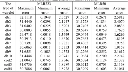
k= σ σ%k− k , respectively.

To choose the proper parameters for wavelet transform, different levels of decomposition and types of wavelets are tested on the simulated data Jasper Ridge. Six levels of wavelet decomposition achieve good performance in this experiment. Two types of wavelet families are implemented, dbN and CoifN wavelets, where N

is the order of the wavelet function. Table 1 lists the maximum error, minimum error and average error of estimation using different wavelets with six levels of decomposition and different number of bands. By comprehensive consideration of the average error, the maximum error and the minimum error, wavelet db5 with six levels of decomposition is chosen in the following experiment.

Table 1 - The errors of estimation using different wavelet with six levels of decomposition and different number of bands.

(8)

6 4 6

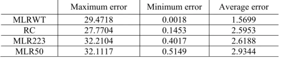
Table 2 - Comparison of the errors of noise estimation by MLRWT, MLR and RC. Maximum error Minimum error Average error

MLRWT 29.4718 0.0018 1.5699

RC 27.7704 0.1453 2.5953

MLR223 32.2104 0.4017 2.6188

MLR50 32.1117 0.5149 2.9344 In the simulated experiment, the comparison between MLRWT and MLR using 223 bands (BIOUCAS-DIAS, et al, 2008) and 50 bands (0.2⋅M , Mis the number of samples) (ACITO, et al, 2011) respectively is performed. Figure 3 shows the difference between the standard deviation of the two methods and the standard deviation of the simulated noise. The result shows that it is important to reduce the spatial correlation by wavelet after the spectral correlation removing step to improve the accuracy of noise estimation. Meanwhile, it shows that MLR223WT obtains a better result. So MLR223WT is referred to as MLRWT, hereinafter.

In order to illustrate the superiority of the proposed algorithm in our paper, our method is also compared with the algorithm RC proposed by Julio (2008). Table 2 lists the estimated standard deviation of the noise in Jasper Ridge by the general MLR using different numbers of bands, RC and MLRWT, respectively.

In the RC method based on classification, the spectral similarity threshold plays an important role in the performance. The spectral angle distance is taken as the spectral similarity threshold in this paper for it is one of the most important parameters to measure the similarity between the two spectrums (KESHAVA and MUSTARD 2002). By previous tuning of the spectral similarity threshold, the RC method obtains an optimal result by the threshold 0.0675 for the Jasper Ridge and the image scene is divided into 61 classes.

On the contrary, MLRWT does not need such tuning, and demonstrates better adaptability and a substantial improvement in the estimation accuracy. By comparing with the general MLR using different numbers of bands, the result shows that wavelet transform reduces the spatial correlation successfully and provide more accurate estimation.

(9)

Figure 3 - The difference between the standard deviation of simulated noise and the estimated standard deviation by MLRWT and MLR. MLR223 and MLR50 mean that the MLR utilizes 223 bands and 50 bands (not including itself)

respectively for regression.

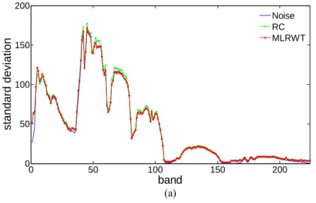
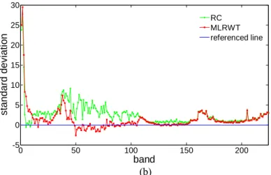
Figure 4 - The estimated noise standard deviation of MLRWT, the general MLR and RC for the Jasper Ridge, (b) the difference between the standard deviation of

simulated noise and the estimated standard deviation by MLRWT and RC.

(a)

0 50 100 150 200

-5 0 5 10 15 20 25 30 35

s

tand

ard d

ev

iat

ion

band

MLR50 MLR223 MLR50WT MLR223WT referenced line

0 50 100 150 200

band

s

tanda

rd devi

a

tion

(10)

6 4 8

(b) 3.2 Real data experiment

The real data experiment of the noise estimation is carried out on Hyperion data (Scene Request ID=EO11280292010303110KF, Site Latitude=+44.1, Site Longitude=+109.6, Date: 03/03/10). The data is from the web: http://datamirror.csdb.cn/. Hyperion covers the 0.4-2.5μm range with 242 spectral bands at approximately 10-nm spectral resolution and 30-m spatial resolution (KRUSE, et al, 2003). As there are some bands in which all the pixel values are zero, these bands are discarded in our experiment. Therefore, the size of datacube we extract from the Hyperion data for testing is 128×128×198 (width ×height × band). Figure 2(b) shows band 40 of this data.

Figure 5 - The estimated noise standard deviation of MLRWT, the general MLR and RC for the Hyperion data. The gaps refer to the bands discarded in the test.

0 50 100 150 200

-5 0 5 10 15 20 25 30

band

s

tand

ard

d

e

v

iati

o

n

RC MLRWT referenced line

0 50 100 150 200

0 20 40 60 80 100 120 140 160 180 200

band

s

tandar

d dev

iat

ion

(11)

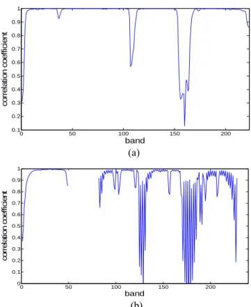
Figure 6 - The spectral correlation coefficient of (a) Jasper Ridge and (b) the Hyperion data. The gaps refer to the bands discarded in the test.

(a)

(b)

Figure 5 is the estimated noise standard deviation of different methods for the real data. It shows that the proposed algorithm MLRWT obtains an available estimation result, which indicates that MLRWT method is feasible.

In both simulated experiment and the real data experiment, it is observed that the performance of estimation in some bands is poor, and the estimated standard deviation in some bands changes sharply, even in the adjacent bands, which is not reliable. The reason for this phenomenon is that the spectral correlation in these bands is weak. The spectral correlation coefficient of band kand k+1 is defined as

1

, , 1

2 1 2

, , 1

( ) ( )

M N

k k

i j k i j k

j i

k

M N M N

k k

i j k i j k

j i j i

x u x u

h

x u x u

+ +

− × −

=

⎛ ₋ ⎞ ⎛_× ₋ ⎞

⎜ ⎟ ⎜ ⎟

⎝ ⎠ ⎝ ⎠

∑∑

(9)

0 50 100 150 200

0.1 0.2 0.3 0.4 0.5 0.6 0.7 0.8 0.9 1

band

c

or

rel

at

ion c

oef

fi

c

ie

nt

0 50 100 150 200

0 0.1 0.2 0.3 0.4 0.5 0.6 0.7 0.8 0.9 1

band

c

or

re

lat

ion c

oef

fi

c

ie

(12)

6 5 0

where uk is the average of pixel values in the k−th bandk=1, 2,..., 223.

Figure 6 shows the spectral correlation coefficient of the Jasper Ridge and the Hyperion data. Compared with the estimated results in Figure 3, Figure 4 and Figure 5, it is shown that when the correlation of bands is weak, the performance of estimation based on MLR is poor. However, due to wavelet transform in spatial domain, our method achieves best results among these methods.

4．CONCLUSION

The significant spectral correlation of hyperspectral remote sensing image is the theoretical basis of using MLR model. Although the spatial correlation of hyperspectral remote sensing image is weaker than the spectral correlation, it can not be ignored, according to which we use the wavelet transform to remove spatial correlation in order to achieve better noise estimation.

In this paper, we carry out simulated experiments of noise estimation on AVIRIS images and real data experiment on Hyperion data. The MLR removes the spectral correlation while the wavelet transform removes the spatial correlation, which guarantees the performance of noise estimation. As the noise estimation based on classification depends on the content of the image, these methods, such as the SSDC, HRDSDC and RC, the improvement of estimation precision is not significant enough. The RC overcomes the defective segmentation process and prevents the same type of Earth objects that are adjacent in one image into two or more different classes. But it is not able to prevent separating the same type of Earth objects that are not adjacent in one image into two or more different classes. In this paper, MRLWT does not require classification, so it has better adaptability. In the simulated experiment the precision of estimation improves over 39% in terms of the average error, compared with the general MLR and RC. The new method also overcomes the insensitivity to the spatial characteristic of the classification methods. In this paper, we only consider the noise term can be properly modelled as additive and spatially stationary. It is reported that the in new-generation hyperspectral sensors the photon noise contribution can not be ignored (Actio, et al, 2011; Uss, et al, 2011), which is not taken account into our method. In future works, we intend to estimate the noise consisting of both dependent and signal-independent terms.

ACKNOWLEDGMENT

This work is supported by the National Natural Science Foundation of China under Project 61101183 and Project 41201363.

BIBLIOGRAPHICAL REFERENCES

(13)

ACITO, N.; DIANI, M.; CORSINI, G. Residual striping reduction in hyperspectral images. 17th International Conference on Digital Signal Processing (DSP),

2011, p. 1-7, 2011.

BIOUCAS-DIAS, J. M.; NASCIMENTO, J. M. P.; Hyperspectral Subspace Identification. IEEE Transactions on Geoscience and Remote Sensing. 46, (8), p. 2435-2445, 2008.

BRUNO A. et al. Noise modelling and estimation of hypersonic data from airborne imaging spectrometers. Annals of Geophysics, 49, (1), p. 1-9, 2006.

CHEN G. Y.; QIAN S. E. Denoising of Hyperspectral Imagery Using Principal Component Analysis and Wavelet Shrinkage. IEEE Transactions on Geoscience and Remote Sensing. 49, (3), p. 973-980, 2011.

DONOHO, D. Nonlinear wavelet methods for recovery of signals, desities, and apectra from in direct and noisy data. Proceeding of Symposia in Applied Mathematics, p. 173-205, 1993.

DONOHO, D. L.; JOHNSTONE, I. M. Threshold selection for wavelet shrinkage of noisy data. Engineering in Medicine and Biology Society, 1994, p. A24-A25, 1994.

GAO, B. C. An operational method for estimating signal to noise ratios from data acquired with imaging spectrometers. Remote Sensing of Environment, 43, (1), p. 23-33, 1993.

GENG X. R.; ZHANG X.; CHEN Z. G. et al. Classification algorithm based on spatial continuity for hyperspectral image. Journal Infrared Millimeter and Waves, , 23, (4), p. 299-302, 2004

RICHARDS J. A.; JIA X. Remote Sensing Digital Image Analysis, Springer-Verlag, Berlin, 1999, Third Edition.

KESHAVA, N.; MUSTARD, J. F.; Spectral unmixing. IEEE Signal Processing Magazine, 19, (1), p. 44-57, 2002.

KRUSE, F. A.; BOARDMAN, J. W.; HUNTINGTON, J. F. Comparison of airborne hyperspectral data and EO-1 Hyperion for mineral mapping. IEEE Transactions on Geoscience and Remote Sensing, 41, (6), p. 1388-1400, 2003 GAO L. R. et al. A New Operational Method for Estimating Noise in Hyperspectral

Images. IEEE Geoscience and Remote Sensing Letters, 5, (1), p. 83-87, 2008. MALLAT, S. G. A theory for multiresolution signal decomposition: the wavelet

representation. IEEE Transactions on Pattern Analysis and Machine Intelligence, 11, (7), p. 674-693, 1989.

JULIO M. J. Comments on “A New Operational Method for Estimating Noise in Hyperspectral Images”. IEEE Geoscience and Remote Sensing Letters, 5, (4), p. 705-709, 2008.

(14)

6 5 2

MIELIKAINEN, J.; TOIVANEN, P. Clustered DPCM for the lossless compression of hyperspectral images. IEEE Transactions on Geoscience and Remote Sensing, 41, (12), p. 2943-2946, 2003.

OTHMAN, H.; QIAN S. E. Noise reduction of hyperspectral imagery using hybrid spatial-spectral derivative-domain wavelet shrinkage. IEEE Transactions on Geoscience and Remote Sensing, 44, (2), p. 397-408, 2006.

ROGER, R. E.; ARNOLD, J. F. Reliably estimating the noise in AVIRIS hyperspectral images. International Journal of Remote Sensing. 17, (10), p. 1951-1962, 1996.