www.the-cryosphere.net/8/689/2014/ doi:10.5194/tc-8-689-2014
© Author(s) 2014. CC Attribution 3.0 License.
The Cryosphere
Modeling near-surface firn temperature in a cold accumulation zone
(Col du Dôme, French Alps): from a physical to a
semi-parameterized approach
A. Gilbert1,2, C. Vincent1,2, D. Six1,2, P. Wagnon2,3,4,5, L. Piard1,2, and P. Ginot2,3,4
1CNRS, LGGE (UMR5183), 38041 Grenoble, France
2Univ. Grenoble Alpes, LGGE (UMR5183), 38041 Grenoble, France 3IRD, LGGE (UMR5183), 38041 Grenoble, France
4IRD, LTHE (UMR5564), 38041 Grenoble, France 5ICIMOD, GPO Box 3226, Kathmandu, Nepal
Correspondence to:A. Gilbert ([email protected])
Received: 11 October 2013 – Published in The Cryosphere Discuss.: 19 November 2013 Revised: 11 February 2014 – Accepted: 4 March 2014 – Published: 17 April 2014
Abstract.Analysis of the thermal regime of glaciers is cru-cial for glacier hazard assessment, especru-cially in the context of a changing climate. In particular, the transient thermal regime of cold accumulation zones needs to be modeled. A modeling approach has therefore been developed to deter-mine this thermal regime using only near-surface boundary conditions coming from meteorological observations. In the first step, a surface energy balance (SEB) model accounting for water percolation and radiation penetration in firn was applied to identify the main processes that control the sub-surface temperatures in cold firn. Results agree well with subsurface temperatures measured at Col du Dôme (4250 m above sea level (a.s.l.)), France. In the second step, a simpli-fied model using only daily mean air temperature and poten-tial solar radiation was developed. This model properly sim-ulates the spatial variability of surface melting and subsur-face firn temperatures and was used to accurately reconstruct the deep borehole temperature profiles measured at Col du Dôme. Results show that percolation and refreezing are ef-ficient processes for the transfer of energy from the surface to underlying layers. However, they are not responsible for any higher energy uptake at the surface, which is exclusively triggered by increasing energy flux from the atmosphere due to SEB changes when surface temperatures reach 0◦C. The
resulting enhanced energy uptake makes cold accumulation zones very vulnerable to air temperature rise.
1 Introduction
on the basis of englacial temperature measurements in the active layer. Although this formulation gives good results and can be used at an annual time step, it requires monthly englacial temperature measurements that are very rare. Even more importantly, it cannot be used for future simulations. Furthermore, investigation of the spatial variability of melt-water refreezing heat flux would require extensive temper-ature measurements, usually not available in the field. Other studies are limited to steady state simulation and do not focus on the relationship between climate and boundary conditions (Aschwanden and Blatter, 2009; Hutter, 1982) or use only time-dependent surface temperature changes imposed by the Dirichlet condition (Lüthi and Funk, 2001; Funk et al., 1993). The aim of this study is to develop a model allowing long-term past and future glacier thermal regime simulations by explicitly taking into account the main surface firn processes such as meltwater percolation and refreezing. To achieve this goal, we could have coupled a thermal regime model to a sophisticated physically based snow model (e.g., CRO-CUS, Brun et al., 1989, 1992). However, this approach re-quires a considerable amount of meteorological data at a short timescale (hour), which is not appropriate for simu-lations to be performed over several decades or centuries. This is why we decided to develop a simple surface tem-perature model suitable for long-term thermal regime sim-ulation based only on daily air temperatures and surface to-pography parameters. The study site and data are presented in Sect. 2. Numerical models are described in Sect. 3 and results are shown and discussed in Sect. 4. Section 4 also ex-plores the spatial variability of surface and englacial temper-atures and applies the model to an example involving deep borehole temperature profiles. The last section presents our conclusions and some future perspectives for this work.
2 Study site and data
2.1 Study site
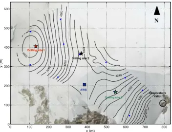
Col du Dôme is located in the Mont Blanc area at an eleva-tion of 4250 m above sea level (a.s.l.). This is a cold accu-mulation zone (Vincent et al., 2007a) on a saddle with slopes of various aspects (Fig. 1). Snow accumulation rates range from 0.5 m w.e. yr−1(meters of water equivalent per year) to
3.5 m w.e. yr−1over short distances (a few hundred meters)
and horizontal surface velocities do not exceed 10 m yr−1
(Vincent et al., 2007b). The mass balance seems to have been stable over the last one hundred years (Vincent et al., 2007b). Mean firn temperature is about −10◦C (below the active thermal layer) but has been significantly rising over the last 20 years due to a recent increase in regional air temperature and surface melting (Gilbert and Vincent, 2013). These tem-perature changes are spatially very variable and dependent on local firn advection velocity, slope, aspect and basal heat flux.
4240
4240
4260 4260
4260
4280
4280
4300 4300
x (m)
y (m)
0 100 200 300 400 500 600 700 800
0 100 200 300 400 500 600
Drilling site 1
AWS
Observatoire Vallot
N
Drilling site 2
Drilling site 3
Fig. 1.Map of Col du Dôme (Mt Blanc range, France) showing the locations of the automatic weather station (AWS; blue square), density measurement sites (blue dots) and borehole drilling sites (stars).
2.2 Field measurements
2.2.1 Meteorological data and firn temperatures
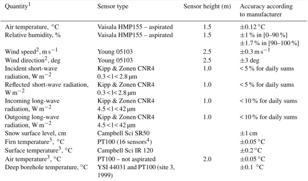
An automatic weather station (AWS) located near the center of the saddle (Fig. 1) ran continuously between 3 July and 23 October 2012. The measurements were carried out within the surface boundary layer. Wind speed, air temperature, hu-midity, incident and reflected short-wave radiation and in-coming and outgoing long-wave radiation were recorded as half-hourly means of measurements made every 10 s (see Ta-ble 1). Instantaneous values of surface position and wind di-rection were collected every half hour. The Vaisala hygro-thermometer was artificially ventilated in the daytime to pre-vent measurement errors due to radiation.
Table 1.List of different sensors of AWS with their specifications.
Quantity1 Sensor type Sensor height (m) Accuracy according
to manufacturer
Air temperature, ◦C Vaisala HMP155 – aspirated 1.5 ±0.12◦C
Relative humidity, % Vaisala HMP155 – aspirated 1.5 ±1 % in [0–90 %]
±1.7 % in [90–100 %]
Wind speed2, m s−1 Young 05103 2.5 ±0.3 m s−1
Wind direction2, deg Young 05103 2.5 ±3 deg
Incident short-wave
radiation, W m−2 Kipp & Zonen CNR40.3 < l < 2.8 µm 1.0 < 5 % for daily sums
Reflected short-wave radiation,
W m−2
Kipp & Zonen CNR4 0.3 < l< 2.8 µm
1.0 < 5 % for daily sums
Incoming long-wave
radiation, W m−2
Kipp & Zonen CNR4 4.5 < l < 42 µm
1.0 < 10 % for daily sums
Outgoing long-wave
radiation, W m−2
Kipp & Zonen CNR4 4.5 < l < 42 µm
1.0 < 10 % for daily sums
Snow surface level, cm Campbell Sci SR50 ±1 cm
Firn temperature3, ◦C PT100 (16 sensors4) ±0.05◦C
Surface temperature3,◦C Campbell Sci IR 120 ±0.2◦C
Air temperature3,◦C PT100 – not aspirated 2.0 ±0.05◦C
Deep borehole temperature,◦C YSI 44031 and PT100 (site 3,
1999)
±0.1◦C
1Quantities are recorded as half-hourly means of measurements made every 10 s except for wind direction and accumulation/ablation, which are
instantaneous values every 30 min.
2Data measurements were interrupted from 12 July 2012 to 6 August 2012 and from 7 October 2012 to 12 October 2012
3Measurement period was 3 July 2012 to 13 June 2013
4Sensor depths are described in Sect. 2.2.1.
2.2.2 Deep borehole temperature profiles
Englacial temperature measurements using a thermistor chain (see Table 1) were performed from surface to bedrock in seven boreholes drilled between 1994 and 2011 at three different sites located between 4240 and 4300 m a.s.l. (Fig. 1). Ice thicknesses were 40, 126, and 103 m at sites 1, 2, and 3, respectively (see Gilbert and Vincent (2013) for more details). Site 1 was measured in January 1999 and March 2012; site 2 in June 1994, April 2005 and March 2010; site 3 in January 1999 and March 2012.
2.2.3 Near-surface densities
On 27 September 2011, density profiles were measured down to a depth of 4 m at 14 different drilling locations at Col du Dôme using a manual auger device (Fig. 1, blue dots).
3 Modeling approach
Two distinct one-dimensional and spatially distributed mod-els are used to calculate the near-surface firn temperatures at Col du Dôme. The first is used to calculate the firn sur-face temperature and melting from a sursur-face energy balance model using the meteorological data recorded by the AWS. The second is a heat flow model coupled to a water
percola-tion model with temperature and melting rate at the surface as input data. This model is used successively with different input data sets obtained first from the energy balance model and then from a parameterized approach.
3.1 Model 1: surface energy balance
A surface energy balance (SEB) model coupled to a one-dimensional heat flow model was developed in order to de-termine the energy fluxes within the firn during the measure-ment period. When heat added by precipitation and penetra-tion of solar radiapenetra-tion are neglected, the SEB equapenetra-tion can be written as (fluxes directed toward the surface are considered positive) (e.g., Oke, 1987)
R+H +LE+Q=Qm (in W m−2), (1)
whereRis the radiative net balance (W m−2),H the
turbu-lent sensible heat flux (W m−2), LE the turbulent latent heat
flux (W m−2), Q the energy flux within the firn (W m−2)and Qmthe energy flux available for melting. The radiative heat
balance is calculated as
R=Sw↓ +Sw↑ +Lw↓ −σ Ts4 (in W m−2), (2)
where Sw↓ is the incident short-wave radiation, Sw↑ the
reflected short-wave radiation, Lw↓ the incoming
emitted by the surface (calculated using the modeled surface temperature Ts and the black body law with
σ=5.67×10⁻⁸W m−2K−4, Essery and Etchevers, 2004).
Turbulent fluxes are explicitly calculated using the bulk aero-dynamic approach, including stability corrections of the sur-face boundary layer (Essery and Etchevers, 2004). Scalar and momentum roughness lengthsz0 are assumed to be equal.
Sincez0has been tuned to match the variation of the internal
energy variation (see Sect. 4.2), selecting a single value forz0
or using distinct values for every roughness length (momen-tum, humidity and temperature) would have changed the val-ues of the roughness parameters, but would not have changed the final results of our simulations. As a consequence, z0
should be considered more as a tuning parameter than as a true roughness length. Sensible and latent heat flux are cal-culated from
H=ρairCpairCHU1(T1−Ts) (3)
LE=LsρairCHU1(Q1−Qsat(Ts, Ps)), (4)
whereρairand Cpairare the density (kg m
−3)and heat
capac-ity (J K−1kg−1)of air, respectively,Q
sat(Ts,Ps)is the
satu-ration humidity at snow surface temperatureTsand pressure Ps,CHis a surface exchange coefficient andLsis the latent heat of sublimation (J kg−1).T
1,Q1andU1are, respectively,
the air temperature (K), the specific humidity (kg kg−1)and
the wind speed (m s−1)at levelz1(m) above the surface. The
exchange coefficient is calculated as a function of the atmo-spheric stability which is characterized by the bulk Richard-son number
Rib=gz1 U12 ×
(T
1−Ts) T1
+Q1−Qsat(Ts, Ps) Q1+ε/(1−ε)
, (5)
whereεis the ratio of molecular weights for water and dry air and g the gravitational acceleration (m s−2).
Then we have the following (Louis, 1979):
CH =fhCHn (6)
with
CHn=km
ln
z
1 z0
−2
(7)
fh=
((1+10R
ib)−1 Rib≥0(stable) (8)
1−10Rib
1
+10CHm(−Rib)1/2
fz
−1
Rib<0(unstable) (9) fz=1/4(
z0 z1)
1/2, (10)
whereCHnis the neutral exchange coefficient for roughness
lenghz0andfha correction factor for atmospheric stability. kmis the Von Karman constant.
The SEB model is coupled to a subsurface model to deter-mine Q (Eq. 1). The one-dimensional heat equation is there-fore solved over a 16 m-deep temperature profile. The up-per surface boundary condition is determined by the SEB
as a flux condition (Neumann) and we assume no heat flux at 16 m depth over the whole simulation period (125 days) (zero-flux boundary condition). This assumption is supported by the fact that over such a short simulation period, basal heat flux has no influence on the modeled temperatures above 10 m depth and consequently it does not have any influence on our results. The time step is set to 5 min (half-hourly meteorological data are linearly interpolated for each time step) and vertical resolution is 4 cm. The heat equation is solved using the Crank–Nicholson scheme. The heat capacity of ice is set to 2050 J K−1kg−1(Paterson, 1994). Densities
have been measured from 0 to 16 m depth into the borehole drilled to install the thermistors. The heat conductivity is cal-culated from density data using the relation from Calonne et al. (2011). The initial temperature profile is taken to be simi-lar to the profile measured at the beginning of the simulation (3 July 2012). Solar radiation penetration is accounted for as-suming that short-wave radiation exponentially decreases as a function of depth (Colbeck, 1989):
FSw(z)=(Sw↓ −Sw↑)∗exp(−z/δ), (11)
whereFsw is the radiative flux at depthzandδ (m) is the
characteristic length of penetration (m).
During the simulation, at every time step, if the surface temperature Ts exceeds 0◦C, Ts is systematically reset to
0◦C, and the temperature difference is used to calculate melt
energy and the resulting volume of meltwater (Hoffman et al., 2008). This amount of energy is then released into the first underlying cold layer below the surface to simulate wa-ter percolation and refreezing. Irreducible wawa-ter saturation (see Sect. 3.2) is taken into account in each model layer. In-deed, when the water content within a model layer exceeds the irreducible water saturation, the remaining water is al-lowed to reach the neighboring underlying layer. All param-eters and variables of model 1 are summarized in Table 2. 3.2 Model 2: coupled water percolation and heat
transfer model
In this second model, Dirichlet conditions are assumed at the surface for temperature and the surface boundary condition for percolation is treated as a water flux. Because the ver-tical resolution of the second model is coarser than that of the previous one (10 cm instead of 4 cm), we assume that the first surface layer is thick enough to absorb all the so-lar radiation. This assumption allows us to take into account the solar radiation penetration, which is here converted into a temperature rise of the surface layer only. In this way, we add a temperatureTrad(K) toTs. Water is assumed to percolate
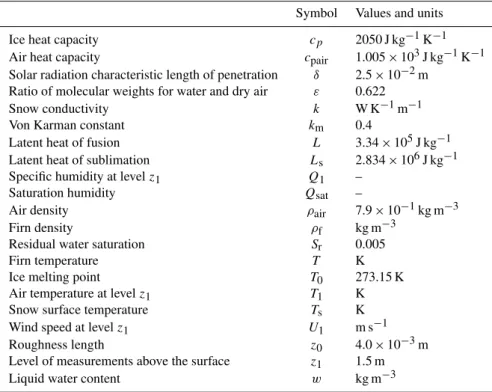
Table 2.Parameters and variables used in the SEB (model 1), with their respective values when available.
Symbol Values and units
Ice heat capacity cp 2050 J kg−1K−1
Air heat capacity cpair 1.005×10³J kg−1K−1
Solar radiation characteristic length of penetration δ 2.5×10⁻²m
Ratio of molecular weights for water and dry air ε 0.622
Snow conductivity k W K−1m−1
Von Karman constant km 0.4
Latent heat of fusion L 3.34×10⁵J kg−1
Latent heat of sublimation Ls 2.834×10⁶J kg−1
Specific humidity at levelz1 Q1 –
Saturation humidity Qsat –
Air density ρair 7.9×10⁻¹kg m−3
Firn density ρf kg m−3
Residual water saturation Sr 0.005
Firn temperature T K
Ice melting point T0 273.15 K
Air temperature at levelz1 T1 K
Snow surface temperature Ts K
Wind speed at levelz1 U1 m s−1
Roughness length z0 4.0×10⁻³m
Level of measurements above the surface z1 1.5 m
Liquid water content w kg m−3
available. We define the effective water saturation S∗:
S∗=S−Sr
1−Sr
, (12)
whereS is the water saturation in the snow, and Sr is the
irreducible water saturation that is permanently retained by capillary forces. IfS<Srthere is no water flow and ifS>Sr,
S∗gravitationally advects and we have
φ (1−Sr) ∂S∗
∂t +nρwgµ
−1KS∗(n−1)∂S∗
∂z =R(in s
−1), (13)
where8 is the porosity, n a constant set to 3.3 (Colbeck and Davidson, 1973),ρw the water density (kg m−3), g
ac-celeration due to gravity (m s−2), µthe viscosity of water
(kg m−1s−1),Kthe intrinsic snow permeability (m2)andR
a negative source term coming from liquid water refreezing (s−1). Snow permeability is calculated as a function of firn
densityρfand mean grain sized (m) using the relationship
from Shimizu (1970):
K=0.077d2exp(−7.8ρf). (14)
The heat advection/diffusion equation is solved and coupled to the water saturation at each time step:
ρfcp
∂T ∂t +vz
∂T ∂z
= ∂ ∂z
k∂T ∂z
+Qlat
in W m−3 (15)
Qlat= mL
1t =R (Lρw8 (1−Sr))
in W m−3, (16)
wherezis the depth (m),t the time (s),T the firn tempera-ture (K),cpthe heat capacity of ice (J kg−1K−1),ρfthe firn
density (kg m−3),v
zthe vertical advection velocity (m s−1),
kthe thermal conductivity of firn (W m−1K−1),Q
latthe
la-tent heat released by refreezing meltwater (W m−3)per unit
of time and volume, m the mass of water that freezes per unit volume (kg m−3)during the time increment 1t (s) and L
the latent heat of fusion (J kg−1). Density variations due to
meltwater refreezing are neglected. Indeed, melting events at such elevation are very rare (not exceeding 10 days per year) and are always punctuated by snowfall events. These lead to a very small density increase.
As proposed by Illangasekare et al. (1990), we impose that m is only a fraction of the maximum water freezing (mmax)allowed by the conservation of heat because in
gen-eral the time step used in modeling will be small compared to the velocity of freezing processes, so we define
w=S8ρw (in kg m−3) (17)
mmax=ρfcp(T0−T )/L (in kg m−3) (18)
m=
(
w, w <dt τfmmax (19)
dt τfmmax, w >dt τfmmax, (20)
wherewis the snow water content (kg m−3),T0the ice
melt-ing point (273.15 K), dt the time step (s) andτfthe freezing
calibration constant (s−1,τ
f< 1 / dt).
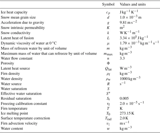
Table 3.Parameters and variables used in the percolation and heat transport model (model 2), with their respective values when available.
Symbol Values and units
Ice heat capacity cp J kg−1K−1
Snow mean grain size d 1.0×10⁻³m
Acceleration due to gravity g 9.81 m s−2
Snow intrinsic permeability K m2
Snow conductivity k W K−1m−1
Latent heat of fusion L 3.34×10⁵J kg−1
Dynamic viscosity of water at 0◦C µ 1.79×10⁻³kg m−1s−1
Mass of refrozen water by unit of volume m kg m−3
Maximum mass of water that can refreeze by unit of volume mmax kg m−3
Water flow constant n 3.3
Porosity 8
Latent heat source Qlat W m−3
Firn density ρf kg m−3
Water density ρw 1000 kg m−3
Water source R s−1
Water saturation S
Effective water saturation S∗
Residual saturation Sr 0.005
Freezing calibration constant τf 2.0×10⁻⁵s−1
Firn temperature T K
Ice melting point T0 273.15 K
Surface temperature correction Trad 2.0 K
Firn advection velocity vz m s−1
Water content w kg m−3
insignificant (approximately of 4.0×10⁻¹W m−2), but
sen-sitivity tests performed with various constant fluxes at 16 m have shown that assuming a zero flux at 16 m does not change the modeled temperature above 10 m depth. The initial tem-perature profile is taken to be similar to the profile measured at the beginning of the measurement period (3 July 2012) and the density profile is set to the one measured on 3 July 2012. This density profile is assumed to be constant over the whole simulation period. The problem is solved numerically using the Elmer/ice finite element model (Gagliardini et al., 2013) based on the Elmer open-source multi-physics package (see http://www.csc.fi/elmer for details) that will make it possible to work in three dimensions and perform thermo-mechanical coupling easily in future studies. Vertical resolution varies from 10 cm near the surface to 40 cm at 16 m depth.
4 Results and discussion
4.1 Meteorological conditions in summer 2012
AWS half-hourly measurements from 3 July 2012 to 23 Oc-tober 2012 are reported in Fig. 2 for wind speed, incoming short- and long-wave radiation, relative humidity, air tem-perature and firn surface temtem-perature. These measurements show 13 days of positive air temperature events, with the warmest event from 15 to 20 August. There were 42 cloudy
days and 69 clear sky days. Based on surface elevation mea-surements, we estimate that three snow falls occurred on 29 August (16 cm), 11 September (30 cm) and 27–28 Septem-ber (15 cm) (Fig. 3). Mean wind speed was 5.4 m s−1, mainly from the southwest and west (> 50 %) with some strong wind events from the northeast. Wind speed and wind direction were unavailable during two periods: 12 July to 6 August and 7–12 October, representing 27 % of the whole measuring pe-riod (Fig. 2). Wind speed was therefore set to its mean value during these periods for energy balance modeling. This ap-proximation is supported by the fact that our simulated sur-face temperatures during this period remain in good agree-ment with measureagree-ments.
4.2 Surface energy balance (model 1)
The calculated temperature and surface melt obtained from the SEB model are reported in Fig. 3. Given that all meltwa-ter refreezes within the cold firn pack, energy is conserved and the modeled energy input should match the energy con-tent variation of the firn pack. For this purpose, the roughness length for momentumz0is tuned so that the measured firn
internal energy matches the modeled energy input (Fig. 4) for every simulation. The energy balance is only adjusted for turbulent fluxes (viaz0) given that the radiative fluxes
Temperature (
°C )
July 15th August 1st August 15th September 1st September 15th October 1st October 15th −20
−15 −10 −5 0
5 0 Relative Humidity (%)
50 100
Incoming short wave radiation (W m
−2
)
0 500 1000
Wind Speed (m s
−1
)
0 5 10 15 20
Surface Temeprature Air Temperatrure
100 200 300 400
Incoming long wave radiation (W m
−2
)
Fig. 2.Meteorological data recorded by the AWS in summer 2012 and surface temperature calculated using measured infra-red surface emissions.
Depth (m)
July 15th August 1st August 15th September 1st September 15th October 1st October 15th −10
−8 −6 −4 −2 0
Temperature (
°C )
−10 −8 −6 −4 −2 0 0
0.7 1.4 2.1 2.8 3.5
Modeled surface melting (mm w.e. h
−1
)
Temperature (
°C )
−30 −20 −10 0
Measured snow surface height variation (m w.e.)
Modeled cumulative surface melting (m w.e.)
−0.05 0 0.05 0.1 0.15 0.2 −10
−5 0
−10 −5 0
Measurements
Model (δ =0 m and Sr = 0)
Model (δ =0.025 m and Sr = 0.005)
Snow fall Snow
fall Melting
NO DATA
a
b
c
e d
24 cm depth 11 cm depth
Surface
Fig. 3. (a)Measured (calculated from long-wave radiation emissions, red line) and modeled surface temperature during summer 2012 at the
AWS withδ=0.0 m andSr=0.0 (blue line) andδ=0.025 m andSr=0.005 (black line).(b, c)Measured and modeled temperature at 11
and 24 cm depth using SEB model(d)Modeled cumulated (black line) and hourly (blue line) surface melting from energy balance compared
Energy ( J m
−2
)
−0.5 0 0.5 1 1.5 2 2.5 3 3.5x 10
7
Water content (kg m
−2)
July 15th Aug 1st Aug 15th Sept 1st Sept15th Oct 1st Oct 15th 0
5 10 15 20 25 30
Measured snow thermal energy variation E
firn − E
0
firn = ∆ Efirn
Modeled energy input Eb
Modeled snow thermal energy variation E
firn − E
0
firn = ∆ Efirn
(Eb − ∆ Efirn) / Lheat
Modeled firn water content in model 2
Fig. 4. (a)Modeled cumulative energy input in firn from surface
energy balance (Eb, blue line), measured and modeled firn thermal
energyEfirn(red and black lines, respectively).(b)Energy
differ-ence between the energy input calculated from the SEB (Eb) and
firn thermal energy (Efirn)compared to modeled water content in
firn using model 2 (integrated on the vertical axis).
comes from turbulent fluxes. The values of radiation pene-tration characteristic lengthδ and water residual saturation
Sr are chosen to minimize RMSE and bias between
mod-eled and measured surface and subsurface temperatures. We find δ=0.025 m that corresponds to the value reported by Brandt and Warren (1993) andSr=0.005, in good agreement
with the model 2 study, where water percolation is investi-gated in more detail (see Sect. 4.3). The corresponding value ofz0that best matches the measured firn internal energy is
4.0 mm. This value is close to the expected value found in the literature at high-altitude cold sites like in Brock et al. (2006) or Wagnon et al. (2003), where roughness lengths have all been chosen equal and also used as tuning parameters.
The calculated hourly surface melt and corresponding cu-mulative melt are displayed in Fig. 3d together with the mea-sured distance between the surface and the SR50 ultrasound sensor expressed as a surface height change in m w.e. using a constant surface density (set to 380 kg m−3)and corrected
according to local air temperature. Two main melting events (25 July to 4 August, and 16 to 26 August) can be
identi-fied and agree fairly well with the surface height variation measurements. The mismatch observed between cumulative surface melt and surface height variations after 1 September may be attributed to wind erosion and fresh snow settlement. Modeled surface temperatures also agree well (r2=0.87, RMSE=1.6 K, bias= −0.02 K, n=5326 half hours) with measured surface temperatures inferred from long-wave ra-diation emissions (Fig. 3a), further supporting the ability of the model to simulate surface melting efficiently. Fig. 3a, b and c compare measured (red line) and modeled surface tem-peratures at 0, 11 and 24 cm depth, respectively, accounting for solar radiation penetration (black line) or not (blue line). When no melting occurs, the cold bias between measurement and model is efficiently attenuated by taking into account so-lar radiation penetration, showing that this effect cannot be neglected at this high elevation cold site, like in cold firn in Greenland (Kuipers Munneke et al., 2009).
Figure 4a compares the integrated thermal energy of the firn pack (red line) obtained from temperature measurements with the modeled energy input (Eb, blue line) obtained from
the model and the modeled firn thermal energy. Firn thermal energyEfirnis calculated from
Efirn=
D Z
0
cp(z)ρf(z)T (z)dz (in J m−2), (21)
whereD(m) is the temperature measurement depth, which is constant over the simulation period, i.e., 16 m at Col du Dôme. Figure 4a shows that energy is conserved except dur-ing the second meltdur-ing event. In this case, the energy input calculated from the SEB exceeds the firn pack thermal en-ergy. Indeed, part of the energy transferred to the firn pack from the surface is stored as latent heat because some firn lay-ers have reached the melting point (Fig. 3e). Consequently, liquid water is stored in the firn (Fig. 4b, blue line). This en-ergy is released when the water refreezes from 17 August to 6 September. This explains why the modeled energy input is once again equal to the firn pack thermal energy several days after the melting event (Fig. 4a).
As illustrated in Fig. 4a, each melting event results in a large energy increase in firn. This means that the surface en-ergy balance is modified during these events. Figure 5 fo-cuses on two consecutive days of melting (18 and 19 Au-gust). During these two days, we compare the energy flux of two cases: (i) a virtual case for which the surface tempera-ture can exceed 0◦C and no melting can occur (dashed lines)
and (ii) the true case for which the surface temperature can-not exceed 0◦C and melting occurs. Note that case (i) is a virtual case where meteorological records have been consid-ered unchanged even though surface temperature is allowed to exceed 0◦C. In reality, meteorological variables such as air
05 H 30 10 H 30 15 H 30 20 H 30 01 H 30 06 H 30 11 H 30 16 H 30 21 H 30 02 H 30 07 H 30 −150
−100 −50 0 50 100 150 200 250 300 350
Times
Energy flux (W m
−2
)
R + LE + S (with melting) R + LE + S (without melting) SW balance LW balance (with melting) LW balance (without melting) Sensible flux (with melting) Sensible flux (without melting) Latent flux (with melting Latent flux (without melting)
Energy excess
Melting period Melting period
Fig. 5.Energy fluxes during two consecutive days of melting (18 and 19 August). Comparison between two cases: (i) no phase change is
taken into account and firn temperature can artificially exceed 0◦C (dashed line); (ii) melting is taken into account (lines and filled blue area).
approach is useful for qualitatively understanding the impact of melting on the SEB over cold surfaces.
In the daytime, for case (i), the short-wave radiative bal-ance is efficiently compensated by the other fluxes due to increasing surface temperature, implying on one hand an en-hanced energy loss due to increased outgoing long-wave ra-diation and on the other hand unstable conditions in the sur-face boundary layer, leading to negative values for sensible heat flux and a strong negative latent heat flux. For case (ii), net short-wave radiation largely dominates the other fluxes because surface temperature cannot exceed 0◦C, thereby limiting heat loss through long-wave radiation and maintain-ing stable conditions inside the surface boundary layer that reduces turbulent fluxes. In this case, a large amount of en-ergy is transferred to the firn. At night, enen-ergy fluxes remain unchanged for both cases. Consequently, the energy uptake during melting events is due to the fact that surface temper-ature is maintained at 0◦C by thermodynamic equilibrium
between the liquid and solid phases.
We conclude that each melting event is associated with a significant energy transfer to the firn pack and the duration of the event therefore has a very strong impact on the total en-ergy balance of the firn pack during summer. With expected higher air temperatures, melting events will become more frequent and the energy will be transferred more efficiently to the firn in the accumulation zones of glaciers. In our case, the strong energy uptake during melting events is less due to melt water percolation and refreezing than to an energy gain in the SEB due to peculiar conditions of the lower atmosphere–firn surface continuum triggered by a 0◦C firn surface. In other
words, for similar atmospheric conditions, firn surfaces are able to absorb more energy when the surface temperature is at 0◦C than when it is negative, explaining why warming of
cold accumulation zones of glaciers is more efficient when melting conditions are encountered than when they are not.
4.3 Subsurface temperature and water content (model 2)
4.3.1 Comparison with data
Measured subsurface temperatures during summer 2012 are shown in Fig. 3e. The influence of surface melting events is clearly visible in the firn temperature data (Fig. 3e). Indeed, we observe a step change in the time evolution of firn temper-ature between 2 and 5 m deep on 25–27 July and 16–18 Au-gust. These temperature increases at these dates are too sharp and rapid to come from diffusive processes and are likely due to additional energy supplied by refreezing meltwater. These observations reveal two striking features: (i) water percolates into cold firn until 4 to 5 m deep and (ii) liquid water crosses the cold firn without totally refreezing.
Model 2 uses the surface temperature and surface melt-ing flux calculated by the SEB model as input data. The only free parameters of the model are the percolation pa-rameters that are not constrained (Sr and τf)and the
con-stant temperature correctionTradof surface temperature
ac-counting for heating due to solar radiation penetration. These parameters were adjusted toτf=2.0×10⁻⁵s−1,Sr=0.005
andTrad=2.0 K, respectively, to match the measured
tem-peratures at all depths (Fig. 6a–e). Figure 4b shows that the modeled water content using model 2 agrees well with the expected value based on the energy balance (see Sect. 4.1). However, the value ofSr is one order of magnitude lower than past published values (Sr=0.03 to 0.07) (Illangasekare
et al., 1990). We think that water does not percolate within the cold firn in a uniform manner but more locally us-ing small preferential pathways (Harrigton et al., 1996), ex-plaining why less water is retained by capillarity in this case. Higher values of Sr lead to more liquid water being
Depth (m)
−8 −6 −4 −2 0
Temperature (
°C )
−11 −10 −9 −8 −7 −6 −5 −4 −3 −2 −1 0
Temperature (
°C )
−10 −5 0 −10 −5 0
−10 −5 0
−10 −5 0
Depth (m)
July 15th August 1st August 15th September 1st September 15th October 1st October 15th −8
−6 −4 −2 0
100 cm
200 cm 65 cm 24 cm
b
c a
d
Forced by daily air temperature from Lyon−Bron (f)
Forced by energy balance model (e)
Fig. 6.Measured (red line) and modeled (blue and black lines) firn temperature at different depths(a, b, c, d). Modeled firn subsurface
temperature during summer 2012 using the energy balance model at a 30 min time step (e, blue line ina, b, c, d) compared to modeled
temperature using the Lyon–Bron temperature at a daily timescale (f, black line inc, d).
prevents water from percolating deep enough to explain the observed firn temperatures. The freezing calibration constant
τfmakes it possible to simulate water percolation in cold firn where only part of the liquid water refreezes between two time steps (30 min here). This parameter is well constrained by our temperature measurements. Indeed, if the value ofτfis
too high, the water will not manage to percolate through cold firn and will not influence the temperature field deep enough compared to measurements. Conversely, if the value ofτfis
too low, the firn temperature never reaches 0◦C and the
en-ergy released by meltwater refreezing is distributed over too large a thickness. The value ofTradshows that it is not
pos-sible to simulate subsurface temperature in snow from sur-face temperature measurements only, because solar radiation partly penetrates into the firnpack. Using a constant correc-tion onTsseems to give satisfactory results.
From these results, we can conclude that our subsurface firn temperature model is able to reproduce the water con-tent and the subsurface temperature field accurately (Figs. 4b and 7). However, this model cannot be applied for simu-lations over several decades or centuries because the half-hourly data it requires are not available over such long peri-ods. Consequently, a simplified approach has been developed with boundary conditions parameterized using daily air tem-perature data.
4.3.2 Simplified approach
For numerical reasons, in order to use a daily time step, the vertical resolution has been reduced from a few centime-ters to about 50 cm. In addition, the previous percolation ap-proach is not meaningful at this space and timescale. For this reason, we now use a constant percolation velocity. The value of 1.0×10⁻⁶m s−1provides the best agreement between the
results obtained with this simplified approach and those with the previous model using the Colbeck and Davidson formu-lation (Fig. 6). All other parameters remained unchanged.
In this way, the boundary conditions are now parameter-ized using the daily mean and maximum air temperatures. Daily surface temperature is assumed to vary in the same way as daily mean air temperature. This is confirmed by one year of hourly simultaneous measurements of surface (infra-red camera) and air temperature at this site (Fig. 7). From these measurements, the mean difference between daily mean air and surface temperature is estimated at 3.4 K (Fig. 7). In order to take into account the enhanced energy uptake dur-ing meltdur-ing events, meltdur-ing is assumed to occur when daily maximum air temperature reaches 0◦C. The daily surface melt flux is calculated using the following degree-day model (Hock, 1999):
M=
(
(Tmax−T0)a, Tmax> T0
0, Tmax≤T0 (in m w.e.d
Sept 2012 Nov 2012 Jan 2013 Mar 2013 May 2013 −35 −30 −25 −20 −15 −10 −5 0 5 Temperature (
°C )
Tair
Ts
−40 −20 0 20
−50 −40 −30 −20 −10 0 10 20
Air temperature ( °C )
Surface temperature (
°C ) T
s = 0.95 * Tair − 3.4
R2 = 0.84
Fig. 7.Comparison between daily measured air (Tair) and surface
(Ts)temperature between 3 July 2012 and 13 June 2013 at Col du
Dôme.
whereM is the daily amount of surface melt (m w.e. d−1), a the melt factor (m w.e. d−1K−1), T0 the melting point (273.15 K) andTmaxthe daily maximum air temperature.
Air temperature data from Lyon–Bron meteorological sta-tion located ∼200 km west of the studied site were lected given that it is one of the longest meteorological se-ries in this region (Gilbert et al., 2012). Comparison between Lyon–Bron air temperature and on-site surface temperature at daily time steps between 3 July 2012 and 13 June 2013 leads to an altitudinal gradient between Lyon air tempera-ture and Col du Dôme surface firn surface temperatempera-ture of
−5.94×10⁻³K m−1. The altitudinal gradient varies
signif-icantly between summer and winter (−5.6×10⁻³K m−1in
winter and−6.5×10⁻³K m−1in summer). As shown
pre-viously, solar radiation penetration cannot be neglected to model firn temperature. As a consequence, the altitudinal gradient selected (or tuned) to reconstruct surface tempera-ture explicitly includes this effect. The constant mean value of−5.9×10⁻³K m−1allows us to match modeled and mea-sured subsurface temperatures. The melt factor is adjusted to simulate the total melt calculated from the SEB during summer 2012 (3 July 2012–23 October 2012) and set to 3.3×10⁻⁴m w.e. d−1K−1. Calculated firn temperatures
us-ing this simplified approach agree well with in situ measure-ments (Fig. 6c, d, f) and properly account for the step change observed during melting events. This reveals that the sim-ple model using daily temperature data from a remote sta-tion provides satisfactory results and can be used to simulate long-term firn subsurface temperature variations in a cold ac-cumulation zone.
4.4 Spatial variability of melting and subsurface temperature
4.4.1 Melting spatial variability
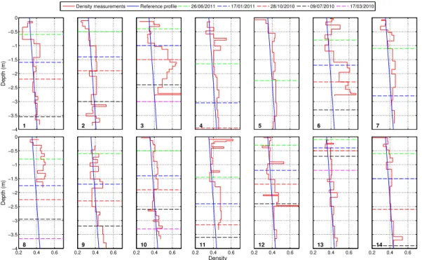
In order to quantify melting spatial variability, 14 4 m-deep density profiles were measured in the field on 27 September 2011 (Figs. 8 and 9). The amount of meltwater was quanti-fied using the density anomaly related to meltwater
refreez-x (m) y (m) 4240 4240 4260 4260 4260 4280 4280 4300 4300 1 2 3 6 5 4 7 8 14 10 9 13 12 11
0 100 200 300 400 500 600 700 800
0 100 200 300 400 500 600
Mean Potential Solar Radiation (W m
−2 ) 150 160 170 180 190 200 210 220 230 240 250 Observatoire Vallot N
Fig. 8.Incoming potential solar radiation at Col du Dôme (color scale). Numbers and blue dots indicate the locations of sites where density measurements were performed. Red stars indicate the loca-tions of sites where snow accumulation has been monitored since 2010. Black square is the location of the AWS.
ing in the firn. This anomaly was quantified in every section of the firn core by comparing the measured density with a computed density obtained from an empirical firn densifica-tion model (Herron and Langway, 1980) (Fig. 9, blue line). Gilbert et al. (2010) successfully applied this method to a high-altitude site in the Andes to quantify local melting. Un-certainty in melt quantification (error bars in Fig. 11) was computed considering uncertainty from mass, length and cir-cumference measurements of each core section. This Col du Dôme site has been monitored for snow accumulation since 1994 using a well-distributed stake network (Vincent et al., 2007b) that provides a good assessment of the spatial vari-ability of snow accumulation at Col du Dôme. In this way, we were able to extrapolate spatially the snow accumulation monitored since 2010 in the vicinity of the measured density profiles (Fig. 8, red stars). Knowing the accumulation rate, we were then able to date every density profile accurately (Fig. 9, dashed lines). Only the density anomaly above the horizon identified on 28 October 2010 has been considered here to make sure that we only take into account the refreez-ing meltwater of summer 2011. The quantified melt at each site is plotted in Fig. 10 as a function of the mean annual in-coming potential solar radiation (PSR) of the corresponding site, taking into account the shading effect of the surrounding relief and atmospheric transmissivity (Fig. 8). Atmospheric transmissivity was determined by comparison of measured short-wave radiation during clear sky conditions with calcu-lated theoretical potential solar radiation and set to 0.78.
−4 −3.5 −3 −2.5 −2 −1.5 −1 −0.5 0
1
Depth (m)
2 3 4 5 6 7
0.2 0.4 0.6 −4
−3.5 −3 −2.5 −2 −1.5 −1 −0.5 0
8
Depth (m)
0.2 0.4 0.6
9
0.2 0.4 0.6
10
0.2 0.4 0.6
11
Density
0.2 0.4 0.6
12
0.2 0.4 0.6
13
0.2 0.4 0.6
14
Density measurements Reference profile 26/06/2011 17/01/2011 28/10/2010 09/07/2010 17/03/2010
Fig. 9.Density profiles (red line) measured on 27 September 2011. Dashed lines correspond to different surface horizons identified at different dates. Blue lines are reference density profiles determined using the empirical model proposed by Herron and Langway (1980).
melt values obtained from the density anomaly method at site 8, 5 m from the AWS. In order to model surface melt over the whole domain using the SEB model, the measured incoming short-wave radiation at AWS is varied artificially according to PSR before re-running the SEB model. In this way we obtain a relationship between surface melt and PSR for summer 2011 from the SEB model. A quadratic func-tion provides a reasonable fit for the melt–PSR relafunc-tionship (Fig. 10). The non-linearity can be explained by the fact that increasing short-wave radiation enhances the frequency and the duration of melting events, which in turn shifts the energy balance towards positive values (see Sect. 4.1).
In order to take into account the effect of PSR on the melting intensity in the degree-day formulation, we revise Eq. (22). PSR is now taken into account in Eq. (23) proposed by Hock (1999) and melt is calculated by
M= (23)
(
(Tmax−T0)aPSR(x, y), Tmax> T0
0, Tmax≤T0
(in m w.e.d−1),
whereaPSRis the melt factor as a function of PSR.
Using daily maximum air temperature inferred from Lyon–Bron daily maximum air temperature (using the same gradient as the one obtained between Lyon–Bron air tem-perature and Col du Dôme surface temtem-peratures in 2012–13) and melt calculated using SEB in summer 2011, we calculate
aPSRfor different PSR values. We found a quadratic
relation-ship (Fig. 10):
aPSR=3.3×10⁻⁸×PSR2−8.23×10⁻⁶
×PSR+5.62×10⁻⁴. (24) In this way, this relationship can be applied to calculate the surface melt and the firn temperature can be calculated us-ing the above-described simplified model for the whole area. However, this relationship is not likely to be transferable to another site. Indeed, melt factors depend on site characteris-tics that influence the surface energy balance such as mean albedo, wind speed, humidity and surface roughness. Thus, the relationship between melt factor and PSR needs to be re-calibrated for every studied site.
4.5 Application of the simplified model at
multi-decennial scale to reconstruct deep borehole temperature profiles
The locations of borehole sites 1, 2 and 3 are indicated on the map in Fig. 1 and their respective annual PSR values are as-sessed at 220, 220 and 192 W m−2. Our simplified 1-D model
(model 2 using daily temperatures from Lyon–Bron station and topographic parameters) was applied to the three sites and run over the period 1907–2012. The vertical advection profile is calculated from the measured surface advection ve-locity and assumed to vary linearly with depth (Gilbert and Vincent, 2013). Basal heat flux is set to 15×10−3W m−2
for sites 1 and 2 and set to 30×10−3W m−2 for site 3
160 180 200 220 240 260 0
2 4 6 8 10 12 14 16 18 20
Potential direct solar radiation (W m−2 )
Summer 2011 surface melt (cm w.e.)
1
3
4
5
6
7 8
9 10 11
12 14
0 0.1 0.2 0.3 0.4 0.5 0.6 0.7 0.8 0.9 1 x 10⁻³
a ( m w.eq.
°C
−1
d
−1
)
Fig. 10.Melt obtained from density anomalies (black stars) as a function of potential solar radiation, compared to melt obtained us-ing the surface energy balance model (red dashed line). Correspond-ing melt factor values in the degree-day model (Eq. 24) are plotted in blue.
heat flux is specified at 150 m depth in the bedrock because it can be considered to be approximately constant at this depth for the timescale of the simulation. The comparison with simulations using a basal heat flux specified at 800 m depth shows that this assumption only influences modeled glacier temperatures below 100 m depth and with a tem-perature difference that does not exceed 0.2 K. The ther-mal properties of the rock (gneiss and granite) are taken from Lüthi and Funk (2001) with a thermal conductivity of 3.2 W m K−1m−1, a heat capacity of 7.5×10²J kg−1K−1
and a density of 2.8×10³kg m−3. The initial temperature
profile in 1907 is calculated as a steady state temperature pro-file. Constant surface steady state temperature for each site is given by Gilbert and Vincent (2013).
For each site, the altitudinal temperature gradient is ad-justed to match observed borehole temperatures. We found values of 5.95×10⁻³, 5.70×10⁻³and 5.83×10⁻³K m−1
for sites 1, 2 and 3 respectively. The respective melt fac-tors for sites 1, 2 and 3 are derived from PSR values (220, 220 and 192 W m−2) and equal to 3.5×10⁻⁴, 3.5×10⁻⁴,
and 2.0×10⁻⁴m w.e. d−1K−1. The results plotted in Fig. 11
show that temperature differences between the three bore-holes can be explained by differences in both surface melt (in agreement with PSR differences) and vertical advection ve-locities. As already seen, PSR has a strong influence on firn temperature of a cold glacier mainly through surface melt and must be accounted for to simulate the thermal regime of cold glaciers. Indeed, site 2 experiences higher surface melting rates than site 3, leading to a stronger firn tem-perature rise over the first decade of this century. Differ-ences between the two sites are amplified by stronger ver-tical advection velocities at site 2. The use of the melt fac-tor specified on the basis of the PSR relationship leads to
−14 −13 −12 −11 −10 −9 −8 −7 −6
−135 −115 −95 −75 −55 −35 −20
Temperature ( °C )
Depth (m)
1994
2005
2010
1999
2011
1999
Site 3
Site 1
Site 2 2011
Fig. 11.Measured (dashed lines and dots) and modeled (solid lines)
temperature profiles at the three drilling sites (site 1=red, site
2=black, site 3=green) for different dates. The blue dashed line
is the temperature profile modeled at site 3 in 1999 and 2012 for a
melt factor set to 1.0×10⁻⁴m w.e. d−1K−1.
modeled temperature in good agreement with measurements for sites 1 and 2 but also to an englacial warming overes-timation of about 0.5◦C for site 3, which is acceptable for
thermal regime simulation at the glacier scale. This over-estimation at site 3 could be corrected by the use of melt-ing factor values of 1.0×10⁻⁴mw. e. d−1K−1 instead of
2.0×10⁻⁴mw. e. d−1K−1(Fig. 11, blue dashed line).
5 Conclusions
accumulation zones become extremely sensitive to climate change. Indeed, when surface temperature reaches 0◦C, the
sum of the radiative and turbulent fluxes shifts towards more positive values, which means that more energy is transferred to underlying layers through water percolating and then re-freezing within cold layers. Consequently, air temperature rise has a very strong impact on temperature profiles in cold glaciers by increasing the frequency and duration of melting events at high elevations. Note that water percolation and re-freezing are very efficient processes for energy transfer from the surface to subsurface firn layers; however, they are not responsible for a higher energy uptake at the surface, which is mainly due to the fact that surface temperature is limited to 0◦C. Our study also highlights the influence of solar
radia-tion penetraradia-tion on firn temperature. Indeed, using measured surface temperature as a Dirichlet condition amounts to ne-glecting radiation penetration, which leads to significant un-derestimation of sub-surface temperature.
To perform numerical simulations over several centuries, instead of applying a sophisticated surface energy balance requiring an excessive amount of data, we also developed a simplified approach based only on daily air temperature and topography. Results from this simplified approach agree well with in situ firn temperature measurements and with results coming from SEB modeling. In addition, if the melt factor is known, this simplified model allows us to reconstruct deep borehole temperature profiles that agree well with measure-ments.
Our measurements show that the spatial variability of melting is highly dependent on the potential solar radiation. This confirms the results obtained by Suter (2002) at these high elevations and we propose a relationship between the melt factor and potential solar radiation at Col du Dôme.
The study of water percolation into the firn shows that gravity flow theory (Colbeck and Davidson, 1973) is suffi-cient to reproduce the observed subsurface temperature by taking into account water flow and refreezing. However, residual saturation in firn must be set to a low value given that water does not percolate uniformly into the cold firn. This may be due to the formation of impermeable ice layers capable of driving water through preferential pathways, leav-ing some parts of the firn pack dry. This results in an apparent residual saturation much lower than expected. However, the gravity flow approach is meaningless at a daily timescale and the use of a constant velocity flow is recommended instead. Although this water percolation scheme is far from reality, it provides good results for subsurface temperature modeling. The same model could be applied in temperate accumulation zones; however, it would be necessary to determine how the water drains at the firn–ice transition.
As the climate is expected to change in the future (IPCC, 2007), cold glacier temperatures will be modified. The re-sponse of subsurface firn temperature to air temperature rise will be largely amplified by an increase in the duration and frequency of melt events. This will lead to strong changes in ice temperature fields. Coupling our surface model with a thermo-mechanical model will make it possible to study the transient response of cold glaciers to climate change and in-vestigate glacier hazards related to thermal regime changes, such as cold hanging glacier stability.
Acknowledgements. This study was funded by the AQWA
Euro-pean program (212250). We are grateful to G. Picard for providing the SEB code and we thank Météo-France for providing Lyon– Bron air temperature data. We thank H. Blatter and R. H. Giesen for helpful comments and suggestions, and we are grateful to H. Harder, who revised the English of this manuscript.
Edited by: M. van den Broeke
The publication of this article is financed by CNRS-INSU.
References
Aschwanden, A. and Blatter, H.: Mathematical modeling and nu-merical simulation of polythermal glaciers, J. Geophys. Res., 114, F01027, doi:10.1029/2008JF001028, 2009.
Brandt, R. E. and Warren, S. G.: Solar heating rates and temperature profiles in Antarctic snow and ice, J. Glaciol., 39, 99–110, 1993. Brock, B. W., Willis, I. C., and Sharp, M. J., Measurement and parameterization of aerodynamic roughness length variations at Haut Glacier d’Arolla, Switzerland, J. Glaciol., 52, 281–297, 2006.
Brun, E., Martin, E., Simon, V., Gendre, C., and Coléou, C.: An energy and mass model of snow cover suitable for operational avalanche forecasting, J. Glaciol., 35, 333–342, 1989.
Brun, E., David, P., Sudul, M., and Brunot, G.: A numerical model to simulate snowcover stratigraphy for operational avalanche forecasting, J. Glaciol., 38, 13–22, 1992.
Calonne, N., Flin, F., Morin, S., Lesaffre, B., Rolland du Roscoat, S., and Geindreau, C.: Numerical and experimental investiga-tions of the effective thermal conductivity of snow, Geophys. Res. Lett., 38 L23501, doi:10.1029/2011GL049234, 2011. Colbeck, S. C.: Snow-crystal growth with varying surface
tempera-tures and radiation penetration, J. Glaciology, 35, 23–29, 1989. Colbeck, S. C. and Davidson, G.: Water percolation through
ho-mogenous snow, The Role of Snow and Ice in Hydrology, Proc. Banff. Symp., 1, 242–257, 1973.
Faillettaz, J., Sornette, D., and Funk, M.: Numerical modeling of a gravity-driven instability of a cold hanging glacier: reanalysis of the 1895 break-off of Altelsgletscher, Switzerland, J. Glaciol., 57, 817–831, 2011.
Funk, M., Echelmeyer, K., and Iken, A.: Mechanisms of fast flow in Jakobshavns Isbrae, Greenland; Part II: Modeling of englacial temperatures, J. Glaciol., 40, 569–585, 1994.
Gagliardini, O., Zwinger, T., Gillet-Chaulet, F., Durand, G., Favier, L., de Fleurian, B., Greve, R., Malinen, M., Martín, C., Råback, P., Ruokolainen, J., Sacchettini, M., Schäfer, M., Seddik, H., and Thies, J.: Capabilities and performance of Elmer/Ice, a new-generation ice sheet model, Geosci. Model Dev., 6, 1299-1318, doi:10.5194/gmd-6-1299-2013, 2013.
Gilbert, A. and Vincent, C.: Atmospheric temperature changes over the 20th century at very high elevations in the European Alps from englacial temperatures, Geophys. Res. Lett., 40, 2102– 2108, doi:10.1002/grl.50401, 2013.
Gilbert, A., Wagnon, P., Vincent, C., Ginot, P., and Funk, M.: Atmospheric warming at a high elevation tropical site revealed by englacial temperatures at Illimani, Bolivia
(6340 m a.s.l., 16◦S, 67◦W), J. Geophys. Res., 115, D10109,
doi:10.1029/2009JD012961, 2010.
Gilbert, A., Vincent, C., Wagnon, P., Thibert, E., and Rabatel, A.: The influence of snowcover thickness on the thermal regime of Tête Rousse Glacier (Mont Blanc range, 3200 m a.s.l.): conse-quences for water storage, outburst flood hazards and glacier response to global warming, J. Geophys. Res., 117, F04018, doi:10.1029/2011JF002258, 2012.
Haeberli, W., Alean, J.-C., Muller, P., and Funk, M.: Assessing risks from glacier hazards in high mountain regions: some experiences in the Swiss Alps, Ann. Glaciol., 13, 96–102, 1989.
Harrington, R. F., Bales, R. C., and Wagnon, P.: Variability of melt-water and solute fluxes from homogeneous melting snow at the laboratory scale, Hydrol. Process., 10, 945–953, 1996.
Herron, M. and Langway Jr., C.: Firn densification: An empirical model, J. Glaciol., 25, 373–385, 1980.
Hock, R.: A distributed temperature-index ice-and snowmelt model including potential direct solar radiation, J. Glaciol., 45, 101– 111, 1999.
Hoffman, M. J., Fountain, A. G., and Liston, G. E.: Sur-face energy balance and melt thresholds over 11 years at Taylor Glacier, Antarctica, J. Geophys. Res., 113, F04014, doi:10.1029/2008JF001029, 2008.
Huggel, C., Haeberli, W., Kääb, A., Bieri, D., and Richardson, S.: An assessment procedure for glacial hazards in the Swiss Alps, Can. Geotech. J., 41, 1068–1083, 2004.
Hutter, K.: A mathematical model of polythermal glaciers and ice sheets. Geophys. Astro. Fluid, 21, 201–224, 1982.
Illangasekare, T. H., Walter, R. J., Meier, M. F., and Pfeffer, W. T.: Modeling of meltwater infiltration in subfreezing snow, Water Resour. Res., 26, 1001–1012, 1990.
Intergovernmental Panel on Climate Change (IPCC), Climate Change 2007: The Physical Science Basis, Contribution of Working Group I to the Fourth Assessment Report of the Inter-governmental Panel on Climate Change„ edited by: Solomon, S., Qin, D., Manning, M., Chen, Z., Marquis, M., Averyt, K. B., Tig-nor, M., and Miller, H. L., Cambridge Univ. Press, Cambridge, UK, 2007.
Louis, J.-F.: A parametric model of vertical eddy fluxes in the atmo-sphere, Bound. Lay. Meteorol., 17, 187–202, 1979.
Lüthi, M. and Funk, M.: Modeling heat flow in a cold, high-altitude glacier: Interpretation of measurements from
Colle Gnifetti, Swiss Alps, J. Glaciol., 47, 314–323,
doi:10.3189/172756501781832223, 2001.
Kuipers Munneke, P., van den Broeke, M. R., Reijmer, C. H., Helsen, M. M., Boot, W., Schneebeli, M., and Steffen, K.: The role of radiation penetration in the energy budget of the snowpack at Summit, Greenland, The Cryosphere, 3, 155–165, doi:10.5194/tc-3-155-2009, 2009.
Oke, T. R.: Boundary Layer Climates, 2nd Edn., 435 pp., Routledge, New York, 1987.
Paterson, W. S. B.: The Physics of Glaciers, 3rd Edn., 480 pp., Perg-amon, New York, 1994.
Ryser, C., Lüthi, M., Blindow, N., Suckro, S., Funk, M., and Bauder, A.: Cold ice in the ablation zone: Its relation to glacier hydrol-ogy and ice water content, J. Geophys. Res.-Earth, 118, 693–705, doi:10.1029/2012JF002526, 2013.
Shimizu, H.: Air permeability of deposited snow, Contributions from the Institute of Low Temperature Science, A22, 1–32, 1970. Skidmore, M. L. and Sharp, M. J.: Drainage system behaviour of a High-Arctic polythermal glacier, Ann. Glaciol., 28, 209–215, 1999.
Suter, S.: Cold firn and ice in the Monte Rosa and Mont Blanc ar-eas:spatial occurrence, surface energy balance and climatic evi-dence, PhD thesis, ETH Zürich, 2002.
Vincent, C., Le Meur, E., Six, D., Possenti, P., Lefebvre, E., and Funk, M.: Climate warming revealed by englacial temperatures at Col du Dôme (4250 m, Mont Blanc area), Geophys. Res. Lett., 34, L16502, doi:10.1029/2007GL029933, 2007a.
Vincent, C., Le Meur, E., Six, D., Funk, M., Hoelzle, M., and Pre-unkert, S.: Very high-elevation Mont Blanc glaciated areas not affected by the 20th century climate change, J. Geophys. Res., 112, D09120, doi:10.1029/2006JD007407, 2007b.
Wagnon, P., Sicart, J.-E., Berthier, E., and Chazarin, J.-P.: Winter-time high-altitude surface energy balance of a Bolivian glacier, Illimani, 6340 m above sea level, J. Geophys. Res., 108, 4177, doi:10.1029/2002JD002088, 2003.
Wilson, N. J. and Flowers, G. E.: Environmental controls on the thermal structure of alpine glaciers, The Cryosphere, 7, 167–182, doi:10.5194/tc-7-167-2013, 2013.
Wright, A. P., Wadham, J. L., Siegert, M. J., Luckman, A., Kohler, J., and Nuttall, A. M.: Modeling the refreezing of meltwater as superimposed ice on a high Arctic glacier: A comparison of approaches, J. Geophys. Res., 112, F04016, doi:10.1029/2007JF000818, 2007.