ACPD
13, 18143–18203, 2013MBL cloud in an LES with bulk aerosol
A. H. Berner et al.
Title Page
Abstract Introduction
Conclusions References
Tables Figures
◭ ◮
◭ ◮
Back Close
Full Screen / Esc
Printer-friendly Version Interactive Discussion
Discussion
P
a
per
|
D
iscussion
P
a
per
|
Discussion
P
a
per
|
Discuss
ion
P
a
per
|
Atmos. Chem. Phys. Discuss., 13, 18143–18203, 2013 www.atmos-chem-phys-discuss.net/13/18143/2013/ doi:10.5194/acpd-13-18143-2013
© Author(s) 2013. CC Attribution 3.0 License.
Atmospheric Chemistry and Physics
Open Access
Discussions
Geoscientific Geoscientific
Geoscientific Geoscientific
This discussion paper is/has been under review for the journal Atmospheric Chemistry and Physics (ACP). Please refer to the corresponding final paper in ACP if available.
Marine boundary layer cloud regimes and
POC formation in an LES coupled to
a bulk aerosol scheme
A. H. Berner1, C. S. Bretherton1, R. Wood1, and A. Muhlbauer2
1
Department of Atmospheric Science, University of Washington, Seattle, Washington, USA
2
Joint Institute for the Study of the Atmosphere and Ocean, University of Washington, Seattle, Washington, USA
Received: 21 June 2013 – Accepted: 25 June 2013 – Published: 8 July 2013 Correspondence to: A. H. Berner ([email protected])
ACPD
13, 18143–18203, 2013MBL cloud in an LES with bulk aerosol
A. H. Berner et al.
Title Page
Abstract Introduction
Conclusions References
Tables Figures
◭ ◮
◭ ◮
Back Close
Full Screen / Esc
Printer-friendly Version Interactive Discussion
Discussion
P
a
per
|
D
iscussion
P
a
per
|
Discussion
P
a
per
|
Discuss
ion
P
a
per
Abstract
A large-eddy simulation (LES) coupled to a new bulk aerosol scheme is used to study long-lived regimes of aerosol-boundary layer cloud-precipitation interaction and the de-velopment of pockets of open cells (POCs) in subtropical stratocumulus cloud layers. The aerosol scheme prognoses mass and number concentration of a single log-normal 5
accumulation mode with surface and entrainment sources, evolving subject to process-ing of activated aerosol and scavengprocess-ing of dry aerosol by cloud and rain.
The LES with the aerosol scheme is applied to a range of steadily-forced simu-lations idealized from a well-observed POC case. The long-term system evolution is explored with extended two-dimensional simulations of up to 20 days, mostly with 10
diurnally-averaged insolation. One three-dimensional two-day simulation confirms the initial development of the corresponding two-dimensional case. With weak mean sub-sidence, an initially aerosol-rich mixed layer deepens, the capping stratocumulus cloud slowly thickens and increasingly depletes aerosol via precipitation accretion, then the boundary layer transitions within a few hours into an open-cell regime with scattered 15
precipitating cumuli, in which entrainment is much weaker. The inversion slowly col-lapses for several days until the cumulus clouds are too shallow to efficiently precipi-tate. Inversion cloud then reforms and radiatively drives renewed entrainment, allowing the boundary layer to deepen and become more aerosol-rich, until the stratocumulus layer thickens enough to undergo another cycle of open-cell formation. If mean sub-20
sidence is stronger, the stratocumulus never thickens enough to initiate drizzle and settles into a steady state. With lower initial aerosol concentrations, this system quickly transitions into open cells, collapses, and redevelops into a different steady state with a shallow, optically thin cloud layer. In these steady states, interstitial scavenging by cloud droplets is the main sink of aerosol number. The system is described in a re-25
ACPD
13, 18143–18203, 2013MBL cloud in an LES with bulk aerosol
A. H. Berner et al.
Title Page
Abstract Introduction
Conclusions References
Tables Figures
◭ ◮
◭ ◮
Back Close
Full Screen / Esc
Printer-friendly Version Interactive Discussion
Discussion
P
a
per
|
D
iscussion
P
a
per
|
Discussion
P
a
per
|
Discuss
ion
P
a
per
|
similar evolutions, except that open-cell formation is phase-locked into the early morn-ing hours.
The same steadily-forced modeling framework is applied to the development and evolution of a POC and the surrounding overcast boundary layer. An initial aerosol perturbation applied to a portion of the model domain leads that portion to transition 5
into open-cell convection, forming a POC. Reduced entrainment in the POC induces a negative feedback between areal fraction covered by the POC and boundary layer depth changes. This stabilizes the system by controlling liquid water path and precipi-tation sinks of aerosol number in the overcast region, while also preventing boundary-layer collapse within the POC, allowing the POC and overcast to coexist indefinitely in 10
a quasi-steady equilibrium.
1 Introduction
Marine stratocumulus clouds cover broad swaths of the world ocean, exerting a strong net radiative cooling effect on climate due to their high albedo (Hartmann et al., 1992). The turbulent circulations maintaining marine stratocumulus are on the order of the 15
boundary layer thickness (1 km), far below the spatial scale resolved by global cli-mate models (GCMs). Marine stratocumulus clouds are thin (100–500 m deep), and are usually capped by a sharp, strong temperature inversion. These sharp gradients are not resolved by GCMs and a challenge to parameterize. They are maintained by strong feedbacks between turbulence, cloudiness, radiation, aerosols and precipitation; 20
in a GCM these are parameterized processes involving substantial subgrid variability. These factors combined make marine stratocumulus a key challenge for simulating cli-mate, including two central uncertainties in simulating anthropogenic climate change – boundary cloud feedbacks (Bony and Dufresne, 2005) and cloud-aerosol interaction (Quaas et al., 2009).
25
ACPD
13, 18143–18203, 2013MBL cloud in an LES with bulk aerosol
A. H. Berner et al.
Title Page
Abstract Introduction
Conclusions References
Tables Figures
◭ ◮
◭ ◮
Back Close
Full Screen / Esc
Printer-friendly Version Interactive Discussion
Discussion
P
a
per
|
D
iscussion
P
a
per
|
Discussion
P
a
per
|
Discuss
ion
P
a
per
usually discussed in terms of the first and second aerosol indirect effects. The first indirect effect (Twomey, 1977) refers to the increase of cloud albedo for constant liquid water path (LWP) when cloud droplet number concentration (Nd) is increased. The second indirect effect (Albrecht, 1989) describes a broader class of feedbacks relating to the impact of changes inNa on Nd and albedo via cloud macrophysical properties 5
such as fractional cloud cover, LWP, and lifetime by means of interactions between microphysical perturbations and cloud dynamics.
Cloud microphysics and dynamics also affect the aerosol. For instance, the droplet collision-coalescence that forms precipitation also reduces aerosol number concentra-tionNa, increasing cloud droplet size and further enhancing precipitation in a positive 10
feedback loop. Baker and Charlson (1990) suggested that this feedback process could lead a cloud layer to evolve toward one of two very different aerosol concentrations (“multiple equilibria”) for a single set of large-scale forcings. Their simple steady state model was based on a mixed layer capped by a stratocumulus cloud of fixed liquid water content (LWC). They predicted marine boundary layer (MBL) aerosol concentra-15
tion given a specified surface aerosol source, treating aerosol sinks due to coagulation, collision-coalescence, and drizzle fall-out. Over a commonly-realized range of aerosol source strengths, their model predicted that an MBL with initialNa below a threshold value would evolve over a few days toward a drizzling state with aerosol concentration
∼10 cm−3 and small cloud albedo, while an MBL with initial Na above the threshold 20
value would evolve toward a non-precipitating state with very high aerosol concentra-tion ∼1000 cm−3 and much larger cloud albedo. Ackerman et al. (1994) approached the same problem using a column model including a cloud layer which responded to the aerosol, parameterized turbulent vertical transports, sophisticated microphysics and radiation. Unlike Baker and Charlson (1990), they found no evidence for bistability, 25
ACPD
13, 18143–18203, 2013MBL cloud in an LES with bulk aerosol
A. H. Berner et al.
Title Page
Abstract Introduction
Conclusions References
Tables Figures
◭ ◮
◭ ◮
Back Close
Full Screen / Esc
Printer-friendly Version Interactive Discussion
Discussion
P
a
per
|
D
iscussion
P
a
per
|
Discussion
P
a
per
|
Discuss
ion
P
a
per
|
An observable manifestation of a positive aerosol-cloud feedback and perhaps bista-bility is the formation of pockets of open cells, or POCs (Stevens et al., 2005), low-albedo regions of cumuliform, open-cellular convection embedded within a sheet of high-albedo closed-cell stratocumulus convection. Early aircraft observations of POCs during the EPIC (Bretherton et al., 2004) and DYCOMS-II (Stevens et al., 2003) field 5
campaigns (Comstock et al., 2005, 2007; van Zanten and Stevens, 2005) documented the contrasts between POCs and surrounding stratocumulus regions. Subsequent ob-servations indicated that the aerosol concentration within POCs is also highly depleted, especially in an “ultraclean layer” just below the inversion (Petters et al., 2006; Wood et al., 2011a). Satellite observations showed POCs form preferentially in the early 10
morning, when stratocumulus cloud is typically thickest and drizzliest, and persist once formed (Wood et al., 2008). The VOCALS Regional Experiment (REx; Wood et al., 2011b) in September–October 2008, targeting the massive and persistent stratocumu-lus deck offthe west coast of Chile, was designed in part to systematically document POC structure. VOCALS Research Flight 06 comprehensively sampled a mature POC 15
one day after its formation, providing an invaluable dataset for modeling and analysis (Wood et al., 2011a). Four other POCs were also sampled by the NCAR/NSF C-130 during VOCALS-REx (Wood et al., 2011b). However, observations alone cannot defini-tively explain how POCs are formed and maintained – this requires a model, and the challenges of resolution and parameterization uncertainties make GCMs nonideal for 20
this task.
Our study focuses on large-eddy simulation (LES) of the MBL as a means to under-stand the complexities of stratocumulus-aerosol-precipitation interaction and their role in POC formation and maintenance. LES of MBL turbulence and clouds explicitly sim-ulate the larger, most energetic eddies that dominate turbulent fluxes. Like GCMs, they 25
ACPD
13, 18143–18203, 2013MBL cloud in an LES with bulk aerosol
A. H. Berner et al.
Title Page
Abstract Introduction
Conclusions References
Tables Figures
◭ ◮
◭ ◮
Back Close
Full Screen / Esc
Printer-friendly Version Interactive Discussion
Discussion
P
a
per
|
D
iscussion
P
a
per
|
Discussion
P
a
per
|
Discuss
ion
P
a
per
Ackerman et al. (2004), which examined the response of a small-domain simulation of marine stratocumulus to specified changes in cloud droplet concentration. Their sim-ulations found a low-aerosol, heavy drizzle regime in which the cloud cover increased and thickened with more aerosol and a higher-aerosol, nearly nondrizzling regime in which the cloud thinned with more aerosol.
5
Recent LES modeling studies in domains with sizes on the order of tens of km have examined the influence of aerosol changes on the ubiquitous mesoscale cellular variability in stratocumulus cloud regimes (Wood and Hartmann, 2006). Some stud-ies focused on cloud response to specifiedNd or aerosol. Savic-Jovcic and Stevens (2008) and Xue et al. (2008) found increased open-cellular organization with decreas-10
ing cloud droplet or aerosol concentration, though the simulations didn’t exhibit as marked a decrease in cloud cover as found in POCs. Berner et al. (2011) simulated the VOCALS-REx RF06 POC case, imposing observationally based Nd differences between the POC and the surrounding overcast region, and reasonably reproduced the observed contrasts in cloud, precipitation and boundary layer structure across the 15
POC boundary. Their simulations also revealed that the overcast region entrained much more strongly than inside the POC, yet the mean inversion height across the domain remained essentially level, with mesoscale circulations compensating the reduced en-trainment in the POC.
A full understanding of the role of aerosol-cloud interactions in the climate sys-20
tem requires simulation of the feedback of cloud processes on aerosols. For this pur-pose, several models have added a simple CCN budget including a number sink due to precipitation-related processes. Mechem and Kogan (2003) used this approach in a mesoscale model (not an LES) with horizontal resolution of 2 km. They simulated transitions from aerosol-rich stratocumulus layers to aerosol-poor, precipitating lay-25
ACPD
13, 18143–18203, 2013MBL cloud in an LES with bulk aerosol
A. H. Berner et al.
Title Page
Abstract Introduction
Conclusions References
Tables Figures
◭ ◮
◭ ◮
Back Close
Full Screen / Esc
Printer-friendly Version Interactive Discussion
Discussion
P
a
per
|
D
iscussion
P
a
per
|
Discussion
P
a
per
|
Discuss
ion
P
a
per
|
Subsequent studies have used LES with simple CCN budgets in mesoscale-size do-mains. Wang and Feingold (2009a) used 300 m (barely eddy-resolving) resolution to look at the evolution of a stratocumulus layer with three initial CCN concentrations, finding sensitivities similar to Mechem and Kogan (2003). Wang and Feingold (2009b) used a 60 km×180 km domain with an initial linear gradient in CCN, showing that the 5
development of open-cell organization smoothly increased as initial CCN decreased. Wang et al. (2010) showed that POCs could be rapidly triggered by reducing the initial aerosol concentration in a mesoscale region within a solid stratocumulus layer, and that the resulting aerosol perturbations and POC structure persist for the 8 h length of their simulation. They also showed that depending on the initial aerosol concentra-10
tion, a stratocumulus-capped boundary layer with the same initial cloud characteristics could either quickly transition into open cells that further reduced aerosol concentra-tion, or persist in a high-aerosol, nearly nonprecipitating state for the length of a 36 h simulation.
Several LES studies have also included more complete models of aerosol processes 15
in cloud-topped boundary layers. Feingold et al. (1996) coupled bin aerosol micro-physics to a 2-D LES and analyzed the role of aqueous chemistry. Feingold and Krei-denweis (2002) explored the effects of different initial aerosol distributions and aque-ous chemistry on cloud dynamics over periods up to eight hours, and coined the term “run-away precipitation sink” for the increasingly efficient removal of aerosol via pre-20
cipitation processes at lower values ofNd. Ivanova and Leighton (2008) implemented a three mode, two moment bulk aerosol scheme within a mesoscale model based on the approximation that aerosol mass within rain or cloud water droplets is proportional to their water mass, but coagulates into one aerosol particle per droplet, as suggested by Flossmann et al. (1985). This approach allows for the inclusion of relatively complete 25
ACPD
13, 18143–18203, 2013MBL cloud in an LES with bulk aerosol
A. H. Berner et al.
Title Page
Abstract Introduction
Conclusions References
Tables Figures
◭ ◮
◭ ◮
Back Close
Full Screen / Esc
Printer-friendly Version Interactive Discussion
Discussion
P
a
per
|
D
iscussion
P
a
per
|
Discussion
P
a
per
|
Discuss
ion
P
a
per
nucleation of new aerosols within the ultraclean layer. Arguably, this is the most real-istic LES depiction of coupled aerosol-stratocumulus cloud-precipitation interactions to date.
In this paper, we build on prior aerosol-cloud-precipitation studies to analyze the multiday evolution and equilibrium states of the coupled stratocumulus cloud-aerosol 5
system subject to a range of constant forcings and initial conditions. For this purpose, we couple a new intermediate-complexity aerosol model to our LES. We recognize that in reality, MBL air is always advecting over a changing SST and subject to changing synoptic forcings and free-tropospheric conditions. However, it is still reasonable to ask whether one can define preferred “regimes” through which the aerosol-cloud system 10
tends to evolve, and if so, whether the system can be expected to evolve smoothly between regimes or whether there are circumstances favoring rapid transitions, or in which the system evolution is sensitive to small changes in the external forcings or initial conditions, and lastly, how such results bear on the aerosol bistability controversy.
Our aerosol model is slightly more complete than schemes which only predict CCN 15
number. It prognoses mass as well as number for a single log-normal accumulation mode, a simplified form of an approach used by Ivanova and Leighton (2008) that is easily coupled into the warm rain portion of the Morrison et al. (2005) double-moment microphysics package used in our LES. Feingold (2003) showed that aerosol geomet-ric mean radius affects the activated fraction of aerosol and thereby aerosol indirect ef-20
fects. In addition to the processes usually included in simple CCN-predicting schemes (parameterized surface source, entrainment from the FT, collision-coalescence, and precipitation fall out), we include interstitial scavenging by cloud and rain, which we find to be an important number sink in less heavily precipitating stratocumulus. Unlike a full-complexity aerosol scheme like that of Kazil et al. (2011), our scheme is still com-25
putationally efficient enough for the extended runs used for the present study, at least when run in two spatial dimensions (2-D).
ACPD
13, 18143–18203, 2013MBL cloud in an LES with bulk aerosol
A. H. Berner et al.
Title Page
Abstract Introduction
Conclusions References
Tables Figures
◭ ◮
◭ ◮
Back Close
Full Screen / Esc
Printer-friendly Version Interactive Discussion
Discussion
P
a
per
|
D
iscussion
P
a
per
|
Discussion
P
a
per
|
Discuss
ion
P
a
per
|
and the aerosol scheme. Section 3 describes how our mostly 2-D simulations are ini-tialized and forced, and Sect. 4 gives an overview of the different simulations. In Sect. 5, we discuss a control simulation which undergoes a transition from closed cell stratocu-mulus to more cumuliform drizzle cells that is qualitatively consistent with observations from the VOCALS field campaign, as well as prior simulations of Mechem and Kogan 5
(2003) and Wang et al. (2010). We also show that a identically forced two-day 3-D run has a qualitatively similar aerosol-cloud evolution as the 2-D control run. Section 6 demonstrates that a small increase in subsidence forcing leads to a stable, overcast equilibrium state instead of the control run evolution, and sensitivity runs test the role of the availability of FT aerosol and the diurnal cycle of insolation. In Sect. 7, we examine 10
a set of identically-forced simulations initialized with different MBL aerosol concentra-tions with a phase plane analysis similar to Bretherton et al. (2010). We use this phase plane to discuss the concept of regimes and their transitions, and we show that there can be multiple equilibria as a function of the initial aerosol state. Finally, in Sect. 8, we use runs initialized with an initial gradient of aerosol concentration to examine the 15
formation of a POC and the subsequent evolution and long-term stability of the coupled system comprised of two cloud regimes – a POC and the surrounding overcast stra-tocumulus. We find that this system can achieve long-term stability due to entrainment feedbacks.
2 Model formulation 20
The simulations in this paper are performed using version 6.9 of the System for At-mospheric Modeling (SAM; Khairoutdinov and Randall, 2003). SAM uses an anelastic dynamical core. Anf-plane approximation with Coriolis force appropriate for the spec-ified latitude is used. In our simulations, the clouds are liquid phase only, and SAM partitions water mass into vapor mixing ratio qv, cloud water mixing ratio qc (drops 25
ACPD
13, 18143–18203, 2013MBL cloud in an LES with bulk aerosol
A. H. Berner et al.
Title Page
Abstract Introduction
Conclusions References
Tables Figures
◭ ◮
◭ ◮
Back Close
Full Screen / Esc
Printer-friendly Version Interactive Discussion
Discussion
P
a
per
|
D
iscussion
P
a
per
|
Discussion
P
a
per
|
Discuss
ion
P
a
per
liquid-ice static energysli=cpT+gz−Lql(neglecting ice). Herecpis the isobaric heat
capacity of air,gis gravity,zis height,Lis the latent heat of vaporization, and the liquid water mixing ratioql is the sum ofqcand qr. Microphysical tendencies are computed using two-moment Morrison microphysics (Morrison and Grabowski, 2008; Morrison et al., 2005), which requires that we also prognose a cloud water number concentra-5
tionNdand a rain number concentrationNr; saturation adjustment is used to repartition betweenqvandqceach time step. We have modified SAM to advect scalars using the selective piecewise-parabolic method of Blossey and Durran (2008), which is less nu-merically diffusive than SAM’s default advection scheme. The 1.5 order TKE scheme of Deardorff(1980) is used as the sub-grid turbulence closure (SGS). The SGS length 10
scale is chosen as the vertical grid spacing, as this inhibits unrealistically large mixing on the highly anisotropic grids (large horizontal relative to vertical spacing) needed to efficiently resolve both the inversion and mesoscale structure in stratocumulus LESs. Surface fluxes are computed in each column from Monin-Obukhov theory. Radiation is calculated every 15 s using the Rapid Radiative Transfer Model (RRTM; Mlawer et al., 15
1997); the solar zenith angle is set for the VOCALS RF06 POC location at 17.5◦S 79.5◦W. Drizzle has been included in the radiation calculation by specifying a com-bined cloud-drizzle water effective radius within each grid cell, computed to give the sum of the optical depths due separately to cloud and drizzle drops in that grid layer.
2.1 Single-mode aerosol scheme 20
We have implemented a new, computationally efficient, single mode, double moment aerosol scheme for warm clouds which tightly couples with Morrison microphysics, in-cluding surface fluxes, entrainment, collision-coalescence, evaporation, and scaveng-ing of interstitial aerosol. The aerosol is described by a sscaveng-ingle log-normal distribution with prognostic mass and number concentration. All the aerosol is assumed to be 25
ACPD
13, 18143–18203, 2013MBL cloud in an LES with bulk aerosol
A. H. Berner et al.
Title Page
Abstract Introduction
Conclusions References
Tables Figures
◭ ◮
◭ ◮
Back Close
Full Screen / Esc
Printer-friendly Version Interactive Discussion
Discussion
P
a
per
|
D
iscussion
P
a
per
|
Discussion
P
a
per
|
Discuss
ion
P
a
per
|
that resides in the condensate particles will correspond to the largest (and hence most easily activated) aerosol particles.
The prognosed aerosol should loosely be thought of as corresponding to the accu-mulation mode. Since we do not represent the Aitken mode, some processes such as spontaneous nucleation of new aerosol particles, or the growth of a population of small 5
aerosol particles via deposition of gasses such as SO2, are not represented. However, the single-mode approximation does capture a variety of important aerosol-cloud in-teraction processes, as we will see, and its simplicity and efficiency make it especially attractive for more idealized simulations.
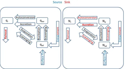
A schematic representation of the various source, sink, and transfer terms for mass 10
and number, considered in the MBL mean, is shown in Fig. 1. We follow the approxi-mation of Ivanova and Leighton (2008) that activated aerosol massqaw is affected by moist processes in proportion to the cloud water massqc, and similarly for rain aerosol massqarvs. rain water massqr:
dqaw
dt |mp=qaw dq
c
dt |mp/qc
, (1)
15
dqar
dt |mp=qar dq
r
dt |mp/qr
, (2)
where|mpdenotes tendencies due to microphysics. Including the effects of aerosol in this way requires prognosing and advecting only four additional scalars, namely dry aerosol number concentration (Nad) and mass mixing ratio (qad) , activated aerosol
20
ACPD
13, 18143–18203, 2013MBL cloud in an LES with bulk aerosol
A. H. Berner et al.
Title Page
Abstract Introduction
Conclusions References
Tables Figures
◭ ◮
◭ ◮
Back Close
Full Screen / Esc
Printer-friendly Version Interactive Discussion
Discussion
P
a
per
|
D
iscussion
P
a
per
|
Discussion
P
a
per
|
Discuss
ion
P
a
per
(unactivated) aerosol, cloud droplets and rain drops:
Na=Nad+Nd+Nr, (3)
qa=qad+qaw+qar. (4)
Ivanova and Leighton included three modes in their scheme: unprocessed aerosol, 5
cloud-processed aerosol, and a coarse mode resulting from evaporated precipitation. By simplifying their approach to a single accumulation mode, we keep the number of auxiliary scalar fields to a minimum. We carry the aerosol mass mixing ratio in addition to number concentration for compatibility with the droplet activation parameterization of Abdul-Razzak and Ghan (2000) used by the Morrison microphysics scheme (which 10
requires these aerosol parameters), and compatibility with a newly developed scaveng-ing parameterization for interstitial aerosol. In the interstitial scheme, described further in the Appendix, scavenging tendencies forqadandNad are computed using the cloud and raindrop size spectra from the Morrison scheme, together with approximate col-lection kernels for convective Brownian diffusion, thermophoresis, diffusiophoresis, tur-15
bulent coagulation, interception, and impaction. While interstitial scavenging has been ignored in several other studies, cloud droplets have a reasonably high collection effi -ciency for unactivated accumulation-mode aerosol (Zhang et al., 2004).
Surface fluxes are computed using a modified version of the wind-speed dependent sea salt parameterization of Clarke et al. (2006), where we have refit the size-resolved 20
fluxes with a single, log-normal accumulation mode. As we are concerned mainly with particles at sizes where they will be viable CCN, we choose to center the source dis-tribution about the geometric radius of 0.13 µm. To include the number and mass con-tributions from the smaller and most numerous portion of the coarse mode, as well as the smallest end of the accumulation mode that may be active CCN at higher super-25
ACPD
13, 18143–18203, 2013MBL cloud in an LES with bulk aerosol
A. H. Berner et al.
Title Page
Abstract Introduction
Conclusions References
Tables Figures
◭ ◮
◭ ◮
Back Close
Full Screen / Esc
Printer-friendly Version Interactive Discussion
Discussion
P
a
per
|
D
iscussion
P
a
per
|
Discussion
P
a
per
|
Discuss
ion
P
a
per
|
CCN.
dNad
dt |Srf=1.706×10 2U
103.41m−2s−1 (5)
dqad
dt |Srf=2.734×10 −19U
103.41kg m−2s−1 (6)
The mass flux is only 0.5 % of that given by Clarke et al. (2006), for which the main 5
mass flux is in large coarse-mode aerosols that again lie outside the range of sizes across which our fit is optimized. Figure 2 plots the size-resolved mass and number fluxes at a windspeed of 9 m s−1 for the Clarke et al. (2006) parameterization against our unimodal approximation.
Aerosol in the free troposphere can be brought into the cloud layer through model-10
simulated entrainment. Observations suggest that over remote parts of the oceans, the FT generally has a substantial number concentration of aerosol particles that can act as CCN (e. g. Clarke, 1993; Clarke et al., 1996; Allen et al., 2011), but these particles usually have diameters significantly smaller than 0.1 microns, and must grow via co-agulation and gas-phase condensation in the boundary layer before they activate into 15
cloud droplets. Because we can not accurately represent this process, we short-circuit it by specifying a free-tropospheric aerosol number concentration comparable to mea-sured CCN concentrations, but by choosing these particles to already have a mean size of 0.1 micron and distribution widthσg=2, similar to what we assume for the surface
aerosol source. Functionally, this is like assuming entrained aerosols instantaneously 20
grow to this mean size by coagulation and gas-phase condensation when they enter the boundary layer, a process which in reality may take hours to days (Clarke, 1993). This assumption also applies to the contribution of number from the surface source at smaller sizes, which we consider as viable CCN when refitting the Clarke et al. (2006) parameterization to our single accumulation mode. Inclusion of nucleation from the gas 25
ACPD
13, 18143–18203, 2013MBL cloud in an LES with bulk aerosol
A. H. Berner et al.
Title Page Abstract Introduction Conclusions References Tables Figures ◭ ◮ ◭ ◮ Back Close
Full Screen / Esc
Printer-friendly Version Interactive Discussion Discussion P a per | D iscussion P a per | Discussion P a per | Discuss ion P a per
The full system of equations governing the bulk aerosol moments in each grid cell are:
dNad
dt =
dNad
dt |Srf−
dNad
dt |Act−
dNad
dt |ScvCld−
dNad
dt |ScvRn+
dNd
dt |Evap+
dNr
dt |Evap
+dNad
dt |NMT (7)
dNd
dt =
dNad
dt |Act−
dNd
dt |Auto−
dNd
dt |Accr−
dNd
dt |Evap+
dNd
dt |NMT (8)
5
dNr
dt =
dNd
dt |Auto−
dNr
dt |SlfC−
dNr
dt |Evap−
dNr
dt |Fallout+
dNr
dt |NMT (9)
dqad
dt =
dqad
dt |Srf−
dqad
dt |Act−
dqad
dt |ScvCld−
dqad
dt |ScvRn+
dqaw
dt |Evap+
dqar
dt |Evap
+dqad
dt |NMT (10)
dqaw
dt =
dqad
dt |Act+
dqad
dt |ScvCld−
dqaw
dt |Auto−
dqaw
dt |Accr−
dqaw
dt |Evap+
dqaw
dt |NMT (11)
dqar
dt =
dqaw
dt |Auto+
dqaw
dt |Accr+
dqad
dt |ScvRn−
dqar
dt |Evap−
dqar
dt |Fallout+
dqar
dt |NMT (12)
10
Here subscript Srf denotes a surface flux, Act is CCN activation, ScvCld is interstitial scavenging by cloud droplets, ScvRn is interstitial scavenging by rain droplets, Evap is evaporation, Auto is autoconversion, Accr is accretion, SlfC is self-collection of rain, and NMT are non-microphysical terms (advection, large scale subsidence, and sub-15
grid turbulent mixing).
The equations for Nd and Nr are identical to the standard implementations within version 3 of the Morrison microphysics implemented in SAM v6.9, though the aerosol mass and number used within the Abdul-Razzak and Ghan activation parameterization are now the local values ofqa=qad+qaw andNad+Nd, respectively. The equation for 20
ACPD
13, 18143–18203, 2013MBL cloud in an LES with bulk aerosol
A. H. Berner et al.
Title Page
Abstract Introduction
Conclusions References
Tables Figures
◭ ◮
◭ ◮
Back Close
Full Screen / Esc
Printer-friendly Version Interactive Discussion
Discussion
P
a
per
|
D
iscussion
P
a
per
|
Discussion
P
a
per
|
Discuss
ion
P
a
per
|
as contributions from the surface flux, interstitial scavenging, and advection/turbulence. The microphysical mass sources and sinks are derived from the corresponding Morri-son cloud and rain mass sources and sinks using the Ivanova–Leighton approximations (1) and (2). One modification was made to the Morrison scheme. The default scheme assumes no loss of cloud droplet number due to evaporation until all water is removed 5
from a grid box (homogeneous mixing). This assumption has been replaced with the heterogeneous mixing assumption that cloud number is evaporated proportionately to cloud water mass, which theory and field measurements suggest may be more appro-priate for stratocumulus clouds (Baker et al., 1984; Burnet and Brenguier, 2007).
The discretized system preserves aerosol mass and number budgets within the do-10
main. The domain-integrated mass source and sink terms are due to surface flux of
qad, fallout ofqar, and mean vertical advection. Aerosol number has a more complex budget. One unforeseen complication was the limiter tendencies within the Morrison microphysics code necessary to prevent unphysical rain and cloud droplet size dis-tributions. To conserve mass, the Morrison scheme adds or subtracts rain and cloud 15
number to keep the droplet size distributions within observationally derived bounds. We maintain a closed aerosol budget under these conditions by shifting aerosol num-ber betweenNrorNdandNad. A spurious source of total number (which we keep track of) can still result from the rare case when the required droplet number source exceeds the available dry aerosol number.
20
2.2 Model domain, grid resolution, and boundary conditions
Most of the simulations were run in two dimensions, as the computational expense of a 10–20 day run was unaffordable in 3-D with readily available resources. In Sect. 5.1, we compare two day periods from identically forced 2-D and 3-D cases, which show qualitatively similar behavior. Except where otherwise noted, 2-D runs use a 24 km 25
ACPD
13, 18143–18203, 2013MBL cloud in an LES with bulk aerosol
A. H. Berner et al.
Title Page
Abstract Introduction
Conclusions References
Tables Figures
◭ ◮
◭ ◮
Back Close
Full Screen / Esc
Printer-friendly Version Interactive Discussion
Discussion
P
a
per
|
D
iscussion
P
a
per
|
Discussion
P
a
per
|
Discuss
ion
P
a
per
30 km (necessary for radiation). One domain-size sensitivity study uses a 96 km wide domain, and the POC runs discussed in Sect. 8 extend the 2-D grid to 192 km in width. The 3-D sensitivity study uses a 24 km×24 km doubly-periodic domain. A dynamical time step of 0.5 s is used in all cases, adaptively shortened when necessary to avoid numerical instability (an infrequent occurrence).
5
3 Initialization and forcing
3.1 Temperature, moisture, and wind
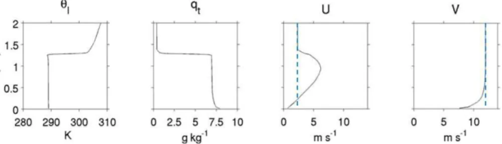
The thermodynamic sounding and winds used in this study are loosely based on the VOCALS-RF06 derived profiles of Berner et al. (2011). Changes include a reduction of the inversion height to 1300 m from 1400 m and initial boundary layerqt reduced to 10
7.0 g kg−1 from 7.5 g kg−1. This results in a thinner and less drizzly initial cloud layer that does not deplete a large fraction of the initial aerosol during the spin-up of the sim-ulations. The wind is forced using a vertically uniform geostrophic pressure gradient and the initial sounding is tuned to minimize inertial oscillations. The free-tropospheric moisture and temperature are nudged to their initial profiles (or downward linear extrap-15
olations thereof, if the inversion shallows more than 150 m from its initial specification) on a one hour timescale in a layer beginning 150 m above the diagnosed inversion height. The sounding and winds averaged over hour three of the control case are de-picted in Fig. 3.
3.2 Radiation 20
ACPD
13, 18143–18203, 2013MBL cloud in an LES with bulk aerosol
A. H. Berner et al.
Title Page
Abstract Introduction
Conclusions References
Tables Figures
◭ ◮
◭ ◮
Back Close
Full Screen / Esc
Printer-friendly Version Interactive Discussion
Discussion
P
a
per
|
D
iscussion
P
a
per
|
Discussion
P
a
per
|
Discuss
ion
P
a
per
|
3.3 Subsidence
Mean subsidence is assumed to increase linearly from the surface to a height of 3000 m and to be constant above that. Throughout this paper, the subsidence profile is in-dicated using its value at a height of 1500 m, which is between 4.75–6.5 mm s−1 in the simulations presented. These values are somewhat larger than our best guess of 5
the actual mean subsidence at 1500 m during VOCALS-RF06 (2 mm s−1; Wood et al., 2011b). This subsidence range was chosen because it exhibits an interesting range of cloud-aerosol-precipitation interaction and long-lived regimes under steady forcing. A simulation with the observed subsidence produces an initial evolution qualitatively similar to the first case discussed below, but with more rapid initial cloud deepening 10
and onset of drizzle. In the VOCALS study region, there is a significant diurnal cycle of subsidence, but we have not included it here for simplicity, since in this paper our focus is on cloud-aerosol regimes which evolve mainly in response to the average forcing over longer periods of time.
3.4 Microphysics
15
The aerosol number concentration in the FT is set to 100 mg−1, typical of FT CCN concentrations over the remote ocean observed in VOCALS (Allen et al., 2011). A sen-sitivity test with no FT aerosol is discussed in Sect. 6.1. Within the MBL, cases with vertically-uniform initial aerosol concentrations ranging from 100 mg−1 to as low as 10 mg−1 are considered, inspired by VOCALS-observed ranges within the MBL over 20
the remote ocean (Allen et al., 2011).
4 Simulations and synopsis of results
ACPD
13, 18143–18203, 2013MBL cloud in an LES with bulk aerosol
A. H. Berner et al.
Title Page
Abstract Introduction
Conclusions References
Tables Figures
◭ ◮
◭ ◮
Back Close
Full Screen / Esc
Printer-friendly Version Interactive Discussion
Discussion
P
a
per
|
D
iscussion
P
a
per
|
Discussion
P
a
per
|
Discuss
ion
P
a
per
line W5/NA100 run, the cloud layer deepens, thickens, and starts to drizzle, transitions to open cellular convection via strong precipitation scavenging, and then collapses; this evolution is also found in a three-dimensional version of this run, as well as in a larger-domain 2-D simulation. IfW is raised to 6.5 mm s−1, the cloud layer deepening is suppressed and a nearly nonprecipitating steady state stratocumulus layer develops. 5
The early development of these runs is reminiscent of prior simulations of Mechem and Kogan (2003) and Wang et al. (2010). A similar bifurcation between cloud thick-ening and collapse vs. development of a steady state is seen when the diurnal cycle is included. For the W6.5 case, we also consider identically forced runs with different initial aerosol concentrations (NA50, NA30, NA10). The NA10 run evolves through an 10
collapsing open-cell regime into a different thin-cloud equilibrium than the other runs. Finally, we consider “POC” simulations in a larger 2-D domain where the initial MBL aerosol includes a horizontal variation in initial MBL aerosol concentration. These runs produce a low-aerosol open-cell state that develops from the initially lowerNaregion, but in the 100 : 50 run, the surrounding region remains a well-mixed, nearly nonprecip-15
itating stratocumulus topped boundary layer with higher aerosol concentrations; this POC-like combined state persists indefinitely given steady forcing.
The model behavior agrees qualitatively with observations in a number of important respects that increase our confidence in its applicability. In the VOCALS campaign, POCs were observed to form rapidly, almost always in the early morning hours when 20
LWP reaches its maximum (Wood et al., 2011b, 2008). In the model, stable stratocumu-lus decks can persist with diurnally averaged LWPs up to around 100 g m−2, but larger LWPs result in precipitation sinks of aerosols that cannot be balanced by reasonable source strengths. This agrees well with the LWP climatology of Wood and Hartmann (2006) for subtropical stratocumulus. The modeled transition from stratocumulus to 25
obser-ACPD
13, 18143–18203, 2013MBL cloud in an LES with bulk aerosol
A. H. Berner et al.
Title Page
Abstract Introduction
Conclusions References
Tables Figures
◭ ◮
◭ ◮
Back Close
Full Screen / Esc
Printer-friendly Version Interactive Discussion
Discussion
P
a
per
|
D
iscussion
P
a
per
|
Discussion
P
a
per
|
Discuss
ion
P
a
per
|
vations, with a surface layer Nad on the order of 20–30 mg−1 and a decoupled upper layer with much lower values, including an “ultra-clean layer” as observed in VOCALS RF06 (Wood et al., 2011b).
5 Evolution through multiple cloud-aerosol regimes
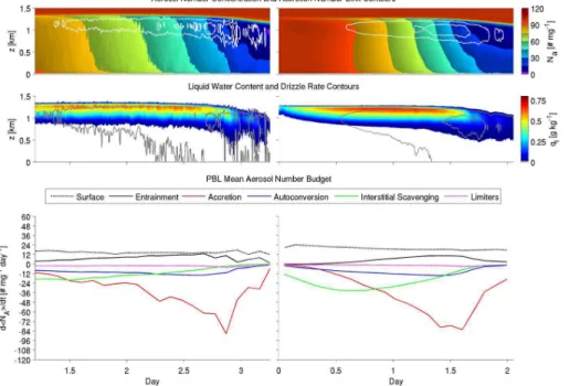
We begin our analysis with run W5/NA100. Figure 4 depicts time-height plots of 5
horizontally-averaged total (dry plus wet) aerosol number concentration and liquid water content, as well as time series for important domain-averaged MBL meteoro-logical variables and for individual tendency terms from the MBL-averaged aerosol number budget. To compute the budget, terms are calculated between the surface and the time-varying horizontal-mean inversion heightzi, determined as the height at 10
which the domain mean relative humidity goes below 50 %. The entrainment source is
we(NaFT−NaMBL)/zi. Here we is the entrainment rate, diagnosed from the difference between the zi tendency and the mean vertical motion at the inversion height. This approach is approximate, but the residual that it induces in the aerosol number budget is only a few percent of the dominant terms. The scavenging of interstitial aerosol num-15
ber by rain is not shown on the aerosol number budget plot, because it never exceeds 1 mg−1day−1, which is much smaller than the terms shown.
The plots reveal three distinct regimes: an initial period with a well-mixed stratocumulus-topped boundary layer, a transitional period with decoupled vertical structure, reduced cloud, and heavy precipitation, and a collapsed boundary layer state 20
with continual weak precipitation and sharply reduced aerosol concentrations.
Over the first two days, the inversion slowly deepens, the stratocumulus layer thick-ens and its LWP increases. There is a 25 % decrease inNadespite relatively negligible surface precipitation. Figure 4d shows that over the first day, the dominant aerosol loss term is interstitial scavenging by cloud, with smaller and roughly comparable losses 25
ACPD
13, 18143–18203, 2013MBL cloud in an LES with bulk aerosol
A. H. Berner et al.
Title Page
Abstract Introduction
Conclusions References
Tables Figures
◭ ◮
◭ ◮
Back Close
Full Screen / Esc
Printer-friendly Version Interactive Discussion
Discussion
P
a
per
|
D
iscussion
P
a
per
|
Discussion
P
a
per
|
Discuss
ion
P
a
per
distribution within defined bounds. These losses are balanced primarily by the surface source, with a slowly increasing contribution from entrainment. As noted by Mechem et al. (2006), the FT may act as a reservoir for MBL CCN when the MBL-average CCN number concentration falls below that of the FT. During the second day, accretion losses begin to rise more sharply, while interstitial scavenging by cloud diminishes. This 5
occurs due to the improved collection efficiency for drizzle drops for constant qr and diminishing Nr, while interstitial scavenging becomes less efficient as cloud droplets grow larger.
During day three, accretion losses grow to dominate the number budget, while Fig. 4c shows entrainment sharply declining as the domain-averaged surface precipitation 10
rate climbs above 0.5 mm day−1. This is an example of what Feingold and Kreiden-weis (2002) called a “runaway precipitation process”. The decrease in entrainment is due to a rapid decrease in turbulence near the top of the boundary layer, because of drizzle-induced stabilization of the boundary layer (Stevens et al., 1998) and reduced destabilization by boundary-layer radiative cooling as cloud cover reduces. The result 15
is a crash of MBLNaand a drastic reduction in LWP. Figure 4d shows the sink terms diminish rapidly at the end of day three, primarily because the vast majority of aerosol has been removed from the cloud layer.
The transition from well-mixed stratocumulus to showery, cumuliform dynamics is abrupt. Figure 5 shows x–z snapshots of ql and Na at three times spanning a six-20
teen hour period (day 2.625 to day 3.295). At the first time, cloud cover is essentially 100 %, withql maxima near 1 g kg−1 and a slight amount of cloud base drizzle under the thickest clouds. Total aerosol concentration Na has only a slight vertical gradient
and is about 40 mg−1in the cloud layer. At the second time, eight hours later, the cloud is thinning and breaking towards the center of the domain, and in a smaller section 25
ACPD
13, 18143–18203, 2013MBL cloud in an LES with bulk aerosol
A. H. Berner et al.
Title Page
Abstract Introduction
Conclusions References
Tables Figures
◭ ◮
◭ ◮
Back Close
Full Screen / Esc
Printer-friendly Version Interactive Discussion
Discussion
P
a
per
|
D
iscussion
P
a
per
|
Discussion
P
a
per
|
Discuss
ion
P
a
per
|
or below 10 mg−1, except for higher values around the strong updraft of the drizzle cell. At the final time, cloud cover has fallen below 50 %; one weak drizzle cell remains, but the cloud layerql is nearly totally depleted. A narrow band of highly depleted aerosol concentrations sits 100–300 m below the inversion, with concentrations falling below 5 mg−1 (an “ultra-clean layer”), while the surface layer concentrations remain between 5
20–30 mg−1. Referring back to Fig. 4d, the net MBL aerosol number sink rate during this 16 h period exceeds 60 mg−1day−1, allowing for near complete aerosol depletion in less than 24 h.
The showery, cumuliform conditions following the sharp transition from stratocumu-lus persist for approximately two days. During this period, Fig. 4c shows that strong 10
drizzle events occur periodically with spikes in surface precipitation up to 4 mm day−1, cloud cover oscillates around 60 % (much of which is optically thin), and domain-mean LWP oscillates between 20–40 g m−2. Entrainment is negligible, so the boundary layer continually shallows and the cumulus cloud layer thins. During the sixth day, surface precipitation becomes lighter and more continuous at around 1 mm day−1, while liquid 15
water path falls to between 10–20 g m−2, as the cloud layer becomes too thin to support episodic cumulus showers. Figure 4a also suggests there is less vertical stratification of the boundary layer aerosol. The boundary layer maintains this state while shallow-ing due to subsidence from a depth of 700 m down to 300 m. This slow boundary layer collapse is reminiscent of results from a one-dimensional turbulence closure modeling 20
study of Ackerman et al. (1993).
After six days of slow collapse, the MBL is sufficiently shallow and the inversion is weak enough that thin cloud forms near the top of the boundary layer and reinvigo-rates entrainment. The sudden influx of entrained aerosol into the cloud decreases cloud droplet sizes, reducing precipitation efficiency and cloud processing sinks within 25
ACPD
13, 18143–18203, 2013MBL cloud in an LES with bulk aerosol
A. H. Berner et al.
Title Page
Abstract Introduction
Conclusions References
Tables Figures
◭ ◮
◭ ◮
Back Close
Full Screen / Esc
Printer-friendly Version Interactive Discussion
Discussion
P
a
per
|
D
iscussion
P
a
per
|
Discussion
P
a
per
|
Discuss
ion
P
a
per
mix the full layer depth, and a decoupled structure takes over with around day 10.5 with lower cloud fraction, slightly reduced entrainment, and a larger vertical aerosol gradient.
The boundary layer continues to deepen and moisten over the next few days with a similar boundary layer structure. On day 15, entrainment begins to strengthen again 5
due to larger LWP and radiatively driven turbulence; full cloud cover is achieved during day 16. While Fig. 4 only extends 20 days, similar simulations we have run past 22 days exhibit limit cycle behavior, collapsing again due to the runaway precipitation sink of aerosol. In a sensitivity test using a 96 km wide domain (run W5/NA100/LD), mesoscale variability allows a region of stratocumulus to form, begin replenishing MBL aerosol, 10
and restart inversion deepening earlier in the collapse process, when the inversion is still at a height of 700 m. This indicates the collapsed regime is fairly delicate in this model.
5.1 Comparison with 3-D results
To check the robustness of our 2-D results, we performed a two-day, 3-D simulation 15
W5/NA100/3-D identical in forcing and initialization to the W5/NA100 case, except us-ing a domain of 24 km×24 km in horizontal extent. The evolution of this run compared with the 2-D control run is depicted in Fig. 6. A few differences are apparent. Entrain-ment in the 3-D simulation is less efficient than in the 2-D run; the boundary layer first shallows during spin-up, then slowly deepens to a maximum of 1270 m after one day 20
of evolution, while the 2-D run is nearly 50 m deeper at this point. This results in less entrainment drying of the boundary layer, and a peak LWP of 175 g m−2is reached in the 3-D case as compared to a maximum of 155 g m−2in the 2-D case. The transition to a collapsing state begins after only 24 h in the 3-D run, while taking 54 h to reach in the 2-D case. This is due partly to the larger LWP accelerating precipitation losses, as well 25
scaveng-ACPD
13, 18143–18203, 2013MBL cloud in an LES with bulk aerosol
A. H. Berner et al.
Title Page
Abstract Introduction
Conclusions References
Tables Figures
◭ ◮
◭ ◮
Back Close
Full Screen / Esc
Printer-friendly Version Interactive Discussion
Discussion
P
a
per
|
D
iscussion
P
a
per
|
Discussion
P
a
per
|
Discuss
ion
P
a
per
|
ing of aerosol within the boundary layer and faster onset of the runaway precipitation sink.
While the strengths of the aerosol number source and sink terms differ quantita-tively between the 2-D and 3-D configurations, their relative roles are similar. Interstitial scavenging is initially the largest sink of Na and the surface flux the largest source. 5
As multiple processes act to reduce Na, the entrainment source strengthens, but is ultimately unable to compete with the accretion losses as drizzle becomes significant. Cloud fraction decreases in both runs following the development of significant surface precipitation and the rainout ofql, demonstrating qualitatively similar dynamics. As the 3-D configuration is nearly 200 times as computationally expensive to run, we use the 10
2-D framework for the remainder of our simulations to enable the long run times nec-essary to examine aerosol-cloud regimes and equilibrium states.
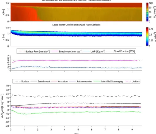
6 Stable equilibrium and sensitivity to forcing
In the W5/NA100 run, cloud breakup occurs when LWP increases enough to induce a runaway drizzle-aerosol loss feedback. This suggests that this transition might be 15
suppressed if LWP remains sufficiently low. With this in mind, Case W6.5/NA100 increases 1500 m subsidence to 6.5 mm s−1, limiting LWP by inhibiting the bound-ary layer from deepening. This case, shown in Fig. 7, reaches a steady, well-mixed, stratocumulus-topped equilibrium state with an inversion height of 1100 m. LWP settles to a mean of approximately 65 g m−2after eight days, with oscillations of±5 g m−2about 20
this value thereafter. The boundary layerNasettles around 88 mg−1, with 100 % cloud cover, less than 0.1 mm day−1 of cloud base drizzle and negligible precipitation reach-ing the surface. The steady state aerosol budget is dominated by an MBL-averaged surfaceNa source of 20 day−1 and an interstitial scavengingNa sink of 12 day−1, with smaller contributions from other processes.
ACPD
13, 18143–18203, 2013MBL cloud in an LES with bulk aerosol
A. H. Berner et al.
Title Page
Abstract Introduction
Conclusions References
Tables Figures
◭ ◮
◭ ◮
Back Close
Full Screen / Esc
Printer-friendly Version Interactive Discussion
Discussion
P
a
per
|
D
iscussion
P
a
per
|
Discussion
P
a
per
|
Discuss
ion
P
a
per
6.1 Sensitivity to FT aerosol
Case W6.5/NA100-0FT is identical to Case W6.5/NA100, except that the FT aerosol concentration is set to zero. In this run, entrainment dilution is always a sink term for MBL-meanNa. After a gradual depletion of aerosol, the run-away precipitation sink
transitions the system into a collapsed MBL. The simulation was run out to 20 days and 5
remained in a collapsed state, with the inversion continually sinking slowly throughout (no plots shown).
6.2 Sensitivity to diurnal cycle of insolation
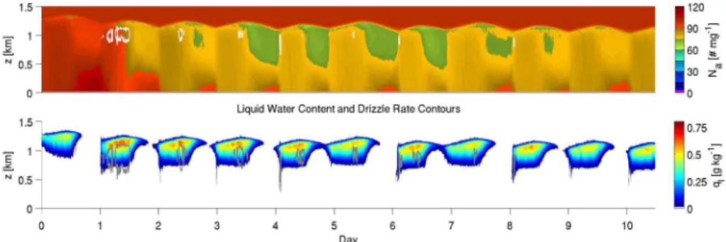
Case W5/NA100/DC (Fig. 8) is configured similarly to the control run W5/NA100, except with a diurnal cycle of insolation. Surprisingly, the inversion does not initially 10
deepen as fast as in the control run, because the daily-mean entrainment rate is lower. This occurs because the cloud dissipates during the daytime, leading to a diurnally-averaged reduction in longwave cooling and turbulence compared to the control case. As a result, the cloud layer evolves towards a steady diurnal oscillation rather than thick-ening until it undergoes the runaway precipitation feedback. The cloud LWP exceeds 15
200 g m−2 for a few hours at night, but this is not long enough for accretion losses to build up before the cloud thins during the daytime and aerosol regenerates. A curious feature of the case is a nearly 2 m s−1oscillation in simulated surface wind speed, driv-ing a large simulated diurnal cycle in surface aerosol number flux(which is proportional to the cube of the wind speed). This effect is attributed to reduced downward turbu-20
lent mixing of momentum to the surface layer during the daytime. Observational data show a much weaker diurnal cycle in windspeed of a few tenths of a meter per second (Dai and Deser, 1999); we speculate that our 2-D approach is artificially amplifying the simulated wind and surface aerosol flux oscillation, although we don’t think this has a major impact on our results. The case was rerun with the 1500 m subsidence rate re-25
ACPD
13, 18143–18203, 2013MBL cloud in an LES with bulk aerosol
A. H. Berner et al.
Title Page
Abstract Introduction
Conclusions References
Tables Figures
◭ ◮
◭ ◮
Back Close
Full Screen / Esc
Printer-friendly Version Interactive Discussion
Discussion
P
a
per
|
D
iscussion
P
a
per
|
Discussion
P
a
per
|
Discuss
ion
P
a
per
|
precipitation is most active, as in the formation of observed POCs (Wood et al., 2008). The sensitivity of the long-term behavior to this slight change in an external parameter is an indicator of a positive-feedback system. The diurnal modulation of the terms in the aerosol number budget does not seem to alter their relative importance in each cloud regime compared to the control case.
5
7 A reduced-order phase-plane description of the aerosol-cloud system
Schubert et al. (1979) discussed characteristic timescales on which a stratocumulus-capped mixed layer adjusts to a sudden change in boundary conditions and forcings. They pointed out that there is a quick (few hours) thermodynamic adjustment of the MBL, followed by a slower adjustment timescale (several days) for the MBL depth to ad-10
just into balance with the mean subsidence. Bretherton et al. (2010) elaborated these ideas using both mixed-layer modeling and LES of stratocumulus-capped boundary layers with fixed cloud droplet concentrations. They showed that with fixed boundary conditions, for any initial condition, the MBL evolution converged after thermodynamic adjustment onto a “slow manifold” along which the entire boundary-layer thermody-15
namic and cloud structure was slaved to a single slowly-evolving variable, the inversion height (zi). With a cloud droplet concentration of 100 cm−3 they found there were two possible slow manifolds, a “decoupled” manifold evolving toward a steady state with small cloud fraction and a shallow inversion, and a “well-mixed” manifold evolving to-ward an solid stratocumulus layer with a deep inversion. In both equilibria, precipita-20
tion was negligible. Simulations initialized with well-mixed boundary layers capped with a cloud layer that was optically thick but non-drizzling converged onto the well-mixed manifold; simulations in which the initial cloud layer was either optically thin or so thick as to heavily drizzle converged onto the decoupled manifold.
In this section, we explore the use of similar concepts for our cloud-aerosol sys-25
ACPD
13, 18143–18203, 2013MBL cloud in an LES with bulk aerosol
A. H. Berner et al.
Title Page
Abstract Introduction
Conclusions References
Tables Figures
◭ ◮
◭ ◮
Back Close
Full Screen / Esc
Printer-friendly Version Interactive Discussion
Discussion
P
a
per
|
D
iscussion
P
a
per
|
Discussion
P
a
per
|
Discuss
ion
P
a
per
its turbulent overturning time of a few minutes (for a coupled boundary layer) to a few hours (for a decoupled boundary layer). Hence, the combination of hNai and zi pro-vides a reduced-order two-dimensional phase-space to describe the “slow manifold” evolution of the cloud-aerosol system on timescales of a day or longer.
We start by viewing the control W5/NA100 case in this way. Figure 10 shows the 5
position inhNai–ziphase space averaged over sequential 12 h periods, colored by the LWP during that period. The first 12 h adjustment period of the vertical structure of the boundary layer and the aerosol is shown in light grey, and the second in dark grey. The spacing between successive points indicates how fast a run is evolving. Diff er-ent “regimes” through which the system evolves are labeled. Here, a cloud-aerosol 10
regime is defined as a part of phase space with qualitatively similar cloud and aerosol characteristics, and hence different balances of terms in the aerosol budget. For in-stance, the open cell regime is characterized by low aerosol, low LWP, low entrainment and efficient precipitation (accretion) removal of aerosol, while the thick cloud regime is characterized by high aerosol, high LWP, little precipitation, high entrainment, and 15
a balance between cloud scavenging and surface/entrainment aerosol sources. The regimes grade into each other ashNaiandzichange; they need not have sharp bound-aries in phase space. The shading indicates two regions of phase-space in which the aerosol concentration evolves comparatively rapidly, either due to runaway precipitation feedback, or due to rapid “runaway” entrainment of aerosol when the shallow boundary 20
layer with open-cell convection redevelops thin inversion-base stratocumulus clouds. Overall, the phase space trajectory has converged onto a limit cycle in which it will indefinitely move between the thick-cloud, open-cell, and thin-cloud regimes.
It is even more interesting to examine the W6.5 case in this framework. The inverted triangles in Fig. 11 show the W6.5/NA100 evolution inhNai–zi phase space. This run 25
shows a slow decrease inzi, with an initial decrease ofhNai, later changing to a slight
increase during the final approach to a “thick-cloud” steady state at zi=1100 m and
ACPD
13, 18143–18203, 2013MBL cloud in an LES with bulk aerosol
A. H. Berner et al.
Title Page
Abstract Introduction
Conclusions References
Tables Figures
◭ ◮
◭ ◮
Back Close
Full Screen / Esc
Printer-friendly Version Interactive Discussion
Discussion
P
a
per
|
D
iscussion
P
a
per
|
Discussion
P
a
per
|
Discuss
ion
P
a
per
|
We performed a sequence of runs identical to W6.5/NA100, but with the initial MBL aerosol concentration varied to 10, 30, and 50 mg−1; results are also plotted on Fig. 11. The simulations with initial Na values of 30 and 50 mg−1 (five and six pointed stars, respectively) evolve to the same thick-cloud equilibrium as the NA100 case. The initial
zi drop is faster for lower hNai, because increased drizzle inhibits entrainment. After 5
a few days, both simulations have settled to nearly their equilibriumzi but still slowly drift toward higherhNaias they approach the steady state.
The run with initialhNaiof 10 mg−1(diamonds) immediately enters a runaway precip-itation feedback as it spins up, transitioning after the first 12 h to a low-LWP collapsing boundary layer. The “elbow” in the lower left corner of the phase space indicates a time 10
at which the MBL eventually recovers a thin layer of stratocumulus and starts to rapidly re-entrain aerosol, as in the W5/NA100 case. In contrast to that case, the stratocumu-lus layer never thickens enough to support vigorous turbulence, and the entrainment is only able to slightly deepen the boundary layer, settling into a second stable “thin-cloud” equilibrium that is different than for the other initial conditions, with highhNaiand 15
no drizzle.
The labelled regimes occupy the same parts of phase space as for W5, because the aerosol loss rate is not directly affected by the instantaneous mean subsidence rate. However, increased subsidence causes individual simulations to evolve through phase space differently than for W5. On Fig. 11, we have sketched in some additional 20
features whose exact structure we can only guess at. The grey and red dashed curves indicates the upper and lower boundaries of attractor basin for the thick-cloud steady state, i. e. all points in phase space from which the slowly-evolving system converges to that steady state. Although the NA50 and NA30 runs appear to start outside this attractor basin, note that it is only after the initial thermodynamic adjustment, which 25

![Fig. 4. Time-heights and time-series for run W5/NA100. (a) Total aerosol number concentration N a with contours [75 225 mg −1 day −1 ] of accretion number sink dN dt d | Accr](https://thumb-eu.123doks.com/thumbv2/123dok_br/16408420.194207/48.918.100.612.70.499/heights-total-aerosol-number-concentration-contours-accretion-number.webp)
![Fig. 5. Left column: x–z cross-sections of liquid water content q l with contours [0.025 0.075 0.125 g kg −1 ] of drizzle water mixing ratio q r](https://thumb-eu.123doks.com/thumbv2/123dok_br/16408420.194207/49.918.99.616.145.403/column-sections-liquid-content-contours-drizzle-water-mixing.webp)