Climate of the Greenland ice sheet using a high-resolution climate model – Part 1: Evaluation

(1)

TCD

4, 561–602, 2010

Part 1: Evaluation

J. Ettema et al.

Title Page

Abstract Introduction

Conclusions References

Tables Figures

◭ ◮

Back Close

Full Screen / Esc

Printer-friendly Version

Interactive Discussion The Cryosphere Discuss., 4, 561–602, 2010

www.the-cryosphere-discuss.net/4/561/2010/ © Author(s) 2010. This work is distributed under the Creative Commons Attribution 3.0 License.

The Cryosphere Discussions

This discussion paper is/has been under review for the journal The Cryosphere (TC). Please refer to the corresponding final paper in TC if available.

Climate of the Greenland ice sheet using

a high-resolution climate model – Part 1:

Evaluation

J. Ettema1, M. R. van den Broeke1, E. van Meijgaard2, W. J. van de Berg1, J. E. Box3, and K. Steffen4

1

Institute for Marine and Atmospheric research Utrecht, Utrecht University, Utrecht, The Netherlands

2

Royal Netherlands Meteorological Institute, De Bilt, The Netherlands

3

Department of Geography, Byrd Polar Research Center, Ohio State University, Columbia, Ohio, USA

4

Cooperative Institute for Research in Environmental Sciences, University of Colorado, Boulder, Colorado, USA

Received: 29 March 2010 – Accepted: 9 April 2010 – Published: 21 April 2010 Correspondence to: J. Ettema (j.ettema@uu.nl)

(2)

TCD

4, 561–602, 2010

J. Ettema et al.

Title Page

Tables Figures

◭ ◮

Back Close

Full Screen / Esc

Interactive Discussion

Abstract

A simulation of 51 years (1957–2008) has been performed over Greenland using the regional atmospheric climate model RACMO2 at a horizontal grid spacing of 11 km forced by ECMWF analysis products. To better represent processes affecting ice sheet surface mass balance, such as melt water refreezing and penetration, an additional

5

snow/ice surface module has been developed and implemented into the surface pa-rameterisation of RACMO2v1. The temporal evolution and climatology of the model is evaluated with in situ coastal and ice sheet atmospheric measurements of near-surface variables and surface energy balance components. The bias for the near-surface air temperature (0.9◦C), specific humidity (0.1 g kg−1), wind speed (0.3 m s−1) as well as

10

for radiative (2.5 W m−2for net radiation) and turbulent heat fluxes shows that the model is in good accordance with available observations. The modeled surface energy bud-get underestimates the downward longwave radiation and overestimates the sensible heat flux. Due to their compensating e_ffect, the averaged 2 m temperature bias is less than−0.9◦C. The katabatic wind circulation is well captured by the model.

15

1 Introduction

The Greenland ice sheet (GrIS) plays a pivotal role in global climate, not only because of its high reflectivity, high elevation, and large area but also because of the volume of fresh water stored in the ice mass equivalent with 7 m global sea level rise. Variations in the surface mass balance (SMB) of the GrIS are determined by the balance between

20

incoming (mass gain) and outgoing (mass loss) terms at the surface. The underlying processes are strongly controlled by atmospheric factors. Therefore, understanding the present-day climate of Greenland is important in the interpretation of the current state and prediction of the future behavior of the ice sheet.

Via multiple feedback mechanisms, changes in ice/snow cover can potentially

(3)

TCD

4, 561–602, 2010

J. Ettema et al.

Title Page

Tables Figures

◭ ◮

Back Close

Full Screen / Esc

Interactive Discussion To quantify these strong nonlinear interactions, extensive observations campaigns are

carried out on the local katabatic circulations and atmospheric boundary layer struc-ture on and around the GrIS (Heinemann, 1999; Oerlemans and Vugts, 1993). In 1996, the climate network GC-net was established with automatic weather stations (AWS) to measure the near-surface atmospheric and surface conditions continuously at

loca-5

tions across the ice sheet (Steffen and Box, 2001).

Whereas these meteorological measurements are limited in space and time, regional climate models have the potential to be used as smart interpolators, yielding useful data for a wide range of times and locations not benefitting from in situ observations. Further, numerical models provide an ideal environment for testing the importance of

10

critical processes in a controlled fashion.

In this study we present the regional atmospheric climate model (RACMO2, Van Mei-jgaard et al., 2008) adapted specially for ice sheet environments. RACMO2 has been successful in simulating surface heat exchange processes and accumulation in Antarc-tica (Van Lipzig et al., 1999; Van de Berg et al., 2006). For Greenland, RACMO2/GR

15

showed that considerably more mass accumulates (up to 63%) for the period 1958– 2007 than previously thought due to the higher horizontal resolution (11 km) and the ice sheet mask that was used. The modeled SMB agrees very well (R=0.95) with the 265 in situ observations that match with the modeled period. Neither the SMB nor the annual precipitation bias shows a spatial coherent pattern, making post-calibration

20

unnecessary (Ettema et al., 2009).

Here, a detailed description and evaluation of RACMO2/GR is presented for the lower atmospheric and surface conditions. The near-surface climatological character-istics of the ice sheet over the period 1958–2008 are described in Ettema et al. (2010). Section 2 describes the model modifications made, which are required to make it

suit-25

(4)

TCD

4, 561–602, 2010

J. Ettema et al.

Title Page

Tables Figures

◭ ◮

Back Close

Full Screen / Esc

Interactive Discussion humidity and surface energy budget component measurements on and along the ice

sheet. Concluding remarks on the model performance are made in Sect. 4.

2 Model description

In this study the Regional Atmospheric Climate Model version 2.1 (RACMO2) of the Royal Netherlands Meteorological Institute (KNMI) is used to simulate the present-day

5

climate of the Greenland ice sheet (GrIS). RACMO2 is a combination of two numerical weather prediction (NWP) models: the atmospheric dynamics originate from the High Resolution Limited Area Model (HIRLAM, version 5.0.6, Und ´en et al., 2002), while the description of the physical processes is adopted from the global model of the European Centre for Medium-Range Weather Forecasts (ECMWF, updated cycle 23r4, White,

10

2004).

At the lateral boundaries, ECMWF Re-Analysis (ERA-40) prognostic atmospheric fields force the model every 6 h, while the interior of the domain is allowed to evolve freely. In the pre-satellite era, the analyses for the Northern Hemisphere benefit from the wide extent of data available from land-based meteorological stations and ocean

15

weather ships. Therefore, the atmospheric forcing for the Arctic area should be well-constrained to start the model simulation in September 1957 (Sterl, 2004; Uppala et al., 2005). After August 2002, operational analyses of the ECMWF have been used to com-plete the model simulation up to January 2009. In absence of an integrated ocean or sea ice model, the open sea surface temperature and sea ice fraction are prescribed.

20

The minimum/maximum model time step is 240/360 s depending on the maximum wind speed in the domain, to ensure numerical stability. The 51-year simulation took approx-imately 100 days on 60 processors of the ECMWF supercomputer.

RACMO2 has 40 atmospheric hybrid-levels in the vertical, of which the lowest is about 10 m above the surface. Hybrid levels follow the topography close to the surface

25

(5)

TCD

4, 561–602, 2010

J. Ettema et al.

Title Page

Tables Figures

◭ ◮

Back Close

Full Screen / Esc

Interactive Discussion nique based on similarity theory applied to the lowest atmospheric model layer (e.g.

Dyer, 1974).

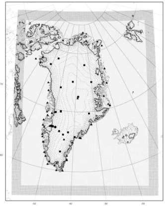
The model domain encompasses the Greenland ice sheet, Iceland, Svalbard, and their neighbouring seas (Fig. 1). The domain includes 312×256 model grid points at a horizontal resolution of about 11 km (0.10 latitudinal degree). This high spatial

5

resolution allows us to resolve much of the narrow ice sheet ablation and percolation zones, as well as the steep climate gradients in the coastal zones. For accurate topo-graphic representation of the GrIS, elevation data and ice mask of the digital elevation model of Bamber et al. (2001) are used. The model surface area of the ice sheet is 1.711×106km2, excluding peripheral ice caps (Fig. 1). This is 1% more than previous

10

studies (Hanna et al., 2008; Box et al., 2006; Fettweis, 2007). Sources of uncertainty include the treatment of changing shelf ice and compacted multi-year sea ice area. The underlying vegetation map is based on the ECOCLIMAP dataset (Masson et al., 2003) and has been manually corrected; the original data set showed too little tundra and too much bare soil along the east coast of Greenland.

15

2.1 Atmospheric model adjustments

General adjustments to the original formulas of the dynamical and physical schemes in RACMO2 are described in detail by Van Meijgaard et al. (2008). Here we only describe the adjustments to the original model formulation that have been made to better represent the melting snow conditions in the Arctic region (RACMO2/GR).

20

RACMO2/GR calculates the surface turbulent heat fluxes from Monin-Obukhov sim-ilarity theory using transfer coefficients based on the Louis (1979) expressions. An effective surface roughness length is used to account for the effect of small scale sur-face elements on turbulent transport. Originally, the roughness lengths for momentum, heat, and humidity (z0m,z0h,z0q) included the effect of enclosing vegetation, urbanisa-25

(6)

TCD

4, 561–602, 2010

J. Ettema et al.

Title Page

Tables Figures

◭ ◮

Back Close

Full Screen / Esc

Interactive Discussion the tundra area without snow and to 1 mm for snow-covered tundra. The value ofz0m

at the snow covered ice sheet is set to 1 mm, whilez0m is set to 5 mm if bare glacier

ice is at the surface. The roughness lengths for heat and humidity over snow sur-faces are computed according to Andreas (1987). This model calculatesl n(z0h/z0m)

orl n(z0q/z0m) as a function of the roughness Reynolds number, R∗=u∗z0/υ, where

5

u∗ is the friction velocity, z0 the roughness length andυthe kinematic viscosity of air. Based on recent observations in the ablation zone, this model is slightly modified for bare ice areas of the ice sheet (Smeets and Van den Broeke, 2008).

Simulations with RACMO2 for the Antarctic region have shown that the original model configuration overestimates liquid precipitation at the expense of solid precipitation

10

(Van de Berg et al., 2006). By imposing that clouds with temperatures below−7◦C form snow only, the solid precipitations flux increases leaving the total precipitation sum unchanged. Due to the much lower air temperatures at the higher elevations, this correction only a_ffects the lowest areas of the ice sheet.

2.2 Snow model 15

The original ECMWF surface scheme (TESSEL; Tiled ECMWF Surface Scheme for Exchanges over land) does not make a distinction between the snow mantle on an ice sheet and seasonal snow cover on the tundra. Snow cover is treated as a single layer on top of the soil or vegetation, which is in thermal contact with the underlying soil. This is acceptable for a transient snow layer over the tundra, but not for the semi-permanent

20

ice sheet firn layer. Snow/firn processes such as melt water percolation, retention and refreezing are not included, while these are especially important to realistically simulate the SMB of an ice sheet with extensive summertime melting (Genthon, 2001).

For a better representation in RACMO2/GR of the processes affecting the SMB, we introduced an additional surface tile “ice sheet” in the land surface scheme TESSEL to

25

(7)

TCD

4, 561–602, 2010

J. Ettema et al.

Title Page

Tables Figures

◭ ◮

Back Close

Full Screen / Esc

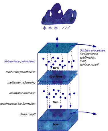
Interactive Discussion at least the upper 30 m with a multi-layer snow/firn/ice model (1-D), in which meltwater

formed at the surface, is allowed to penetrate to deeper layers, where it may refreeze (internal accumulation) or runoffas described by Bougamont et al. (2005).

The optimal thickness of a snow/firn/ice layer increases linearly from 6.5 cm for the uppermost layer to 4 m for the lowermost layer. The layer thickness is continuously

5

changing due to snow accumulation, sublimation/deposition, melting, internal accu-mulation and firn densification. The vertical grid is adjusted by layer splitting when the layer thickness becomes more than 1.3 times its optimal thickness, or layer fusion when a layer is less than half of its optimal thickness, except for layers consisting of ice lenses in the firn.

10

Snow/firn densityρchanges due to refreezing of capillary water (rain and meltwater) and the settling and packing of dry snow according to the empirical formulation by Herron and Langway (1980):

forρ < 550 kg m−3: dρ

dt =k0a(ρi−ρ) (1)

withk0=11exp

−10160 RT

15

for 550 kg m−3 ≤ρ < 800 kg m−3: dρ dt =k1a

0.5

(ρ_i−ρ) (2)

withk1=575exp

−21400 RT

where a is the annual accumulation rate, R the universal gas constant, and T the firn/snow temperature in K. The annual accumulation rate used in this formula is the

20

spatially distributed accumulation averaged over the period 1989–1995 based on an earlier 16-year integration with RACMO2/GR.

The snow/firn/ice column is thermally coupled to the atmospheric part of RACMO2/GR through a surface skin layer formulation of the surface energy balance (SEB) and the surface albedo,α.

(8)

TCD

4, 561–602, 2010

J. Ettema et al.

Title Page

Tables Figures

◭ ◮

Back Close

Full Screen / Esc

Interactive Discussion The surface-atmosphere interface is infinitely thin having no heat capacity and

re-sponding instantaneously to SEB changes. The skin temperatureTsis solved by SEB

closure (e.g. Brutsaert, 1982):

m=SW_net+LW_net+SHF+LHF+Gs

=SW_↓(1−α)+LW_↓−ǫσT4

s 5

+SHF+LHF+G_s (3)

whereM is the melt energy, SW↓, SW↑, LW↓, LW↑the downward and upward directed

fluxes of solar and longwave radiation,αthe broadband surface albedo,ǫthe surface emissivity for longwave radiation (ǫ=0.98 in RACMO2/GR for the ice sheet), σ the Stefan-Boltzmann’s constant, LHF and SHF the turbulent fluxes for latent and sensible

10

heat, andG_s the subsurface conductive heat flux at the surface. All terms are defined as positive when directed towards the surface-atmosphere interface.

The skin temperature serves as boundary condition to the englacial module, which treats the vertical conduction of heat as follows:

ρc_p∂T

∂t =−

∂ ∂z

k∂T

∂z

+Q= +∂G

∂z +Q (4)

15

whereρ is the density of the snow/firn/ice layer, c_p the specific heat capacity of ice (2009 J kg−1K−1),∂T/∂tthe rate of temperature change within one model time step,k

the effective conductivity,zthe vertical coordinate, andQthe heat released by refreez-ing of melt water. The term∂G/∂zaccounts for the heat diffusion driven by the vertical temperature gradient. The snow/firn/ice conductivity follows the density-dependent

ap-20

proach of Van Dusen (1929), which ensures the correct value for k if ice density is attained. Temperature dependence ofk is neglected:

k=2.1×10−2₊4.2×10−4ρ+2.2×10−9ρ3 (5)

(9)

TCD

4, 561–602, 2010

J. Ettema et al.

Title Page

Tables Figures

◭ ◮

Back Close

Full Screen / Esc

Interactive Discussion ice and the remaining energy is used for melting. Meltwater and rain are allowed to

percolate into the firn until they refreeze or run o_ff. The maximum retention capacity due to capillary forces is set to a low value of 2% of available pore space, to obtain a realistic densification rate by refreezing of capillary water (Greuell and Konzelman, 1994). If an ice surface is encountered, the remaining water runs o_ffat the surface, or

5

deep in the firn pack at the snow/ice transition without delay.

The snow/firn/ice albedo α follows the snow density ρ and cloudiness n depen-dent linear formulation of Greuell and Konzelman (1994) for the uppermost 5 cm of the snow/firn/ice pack.

α=αi+(ρ1−ρi)

(α_s−α_i) (ρs−ρi)+

0.05(n−0.5) (6)

10

where the subscripti denotes ice and subscriptsdenotes snow. This parameterization is based on the notion that density reflects the metamorphosis state of the snow, i.e. it represents mostly the effects of grain size on albedo. Fresh snow is characterized by a surfaceα of 0.825 and a density of 300 kg m−3. Glacier ice has an albedo of 0.5 and a density of 900 kg m−3. Refrozen melt water or rain may increase the density of the

15

firn pack to the ice density, but the surface albedo is limited to a minimum value of 0.7 for refrozen water (Stroeve et al., 2005). This limitation will mainly affect areas south of 70◦N, where daytime melt and nighttime refreezing occurs regularly throughout the melt season.

2.3 Model initialization 20

The atmospheric prognostic profiles of temperature, specific humidity, wind speed, and surface pressure are initialized from ERA-40 at the beginning of the integration. By starting the simulation at the end of the melting season, the tundra could realistically be prescribed as snow free. Over the ice sheet, it is important to initialize the snow/ice temperature and snow/firn density with fairly realistic profiles, since typical timescales

25

(10)

TCD

4, 561–602, 2010

J. Ettema et al.

Title Page

Tables Figures

◭ ◮

Back Close

Full Screen / Esc

Interactive Discussion Initial temperature and density profiles of the snow/firn/ice column were obtained by

rerunning the first model year (1 September 1957 to 31 August 1958) three times. The first spin-up run started with uniform vertical profiles for snow and ice temperature as described by Reeh (1991), who derived a surface snow/ice temperature parameteriza-tion based on air temperature data from DMI staparameteriza-tions at the periphery of the ice sheet

5

for the 1951–1961 period.

T=T2 m+δT (7)

with T2 m=48.83−0.007924E−0.7512L

δT =0.86+26.6(SIF−0.038)

10

where T is the initial ice temperature in ◦C, T2 m the 2 m air temperature in

◦

C that depends on elevation E and latitude L, and δT a pertubation due to the amount of superimposed ice formed, SIF. For SIF, the melt rate is taken averaged over the period 1989–1995 based on an earlier 16-year integration with RACMO2/GR.

In the central region of the ice sheet, the dry-snow zone, where melting is rare, the

15

mean air temperature is a reasonable approximation (within 2◦C) for the climatological deep snow and ice temperature. For the percolation and ablation zones, a temperature correctionδT due to refreezing energy is included in line with Reeh (1991), and the ice temperature is limited to 0◦C. The resulting deep ice temperature serves as boundary condition for lowest firn/ice layer, so no heat flux is allowed to the underlying ice or soil.

20

(11)

TCD

4, 561–602, 2010

J. Ettema et al.

Title Page

Tables Figures

◭ ◮

Back Close

Full Screen / Esc

3 Observational data

A proper evaluation of RACMO2/GR is essential before its output can be used as a tool for studying the climate of Greenland and the recent changes thereof. Moreover, identification of model deficiencies may help to improve the model formulation for future climate simulations. To verify the model results for the near-surface conditions, we use:

5

i) near-surface air temperature and wind speed data from automatic weather stations (AWSs) on the ice sheet (GC-net; Steffen and Box, 2001) and from synoptic stations on the surrounding tundra of the Danish Meteorological Institute (DMI), ii) data on near-surface climate, near-surface radiation and heat exchange processes from three K-transect AWSs (Van den Broeke et al., 2008b,a).

10

Statistical procedures were applied to all observational data sets to remove occa-sional spurious data values. For model evaluation of monthly means, we require that at least 80% of the observations are available during one month. The length of an observational record does not influence the evaluation, since every separate month is compared independently with the same month from the model output. The elevation

15

of model grid points closest to all observational sites is within 100 m of the observed elevation, suggesting that no height correction is needed for temperature.

3.1 GC-net

The Greenland Climate Network (GC-net) was started in 1995 and has consisted until 2001 of 15 AWSs (indicated as squares in Fig. 1) near or above the 2000 m elevation

20

contour. Station coordinates and detailed information on the measurements is given in Steffen and Box (2001). We obtained a complete and quality controlled dataset for the period 1998–2001.

Three parameters derived from direct observations are compared with the RACMO2/GR output: air temperature, wind speed and net shortwave radiation, as

25

(12)

inter-TCD

4, 561–602, 2010

J. Ettema et al.

Title Page

Tables Figures

◭ ◮

Back Close

Full Screen / Esc

Interactive Discussion polation. A logarithmic wind profile is assumed with a roughness length of 0.5 mm to

estimate the 10 m wind speed. Due to riming of the sensors, net solar radiation data are omitted for the springtime months March and April. The available net radiation ob-servations are excluded in this study, because these unventilated measurements often su_ffer from large errors due to riming inside and outside the polyethylene domes. Only

5

the net radiation records of the sites Swiss Camp and JAR1 are believed to be reliable throughout the year.

3.1.1 K-transect

In parallel with the GC-net, UU/IMAU installed three AWSs along the Kangerlus-suaq transect (K-transect) in southwest Greenland in August 2003 (Van den Broeke

10

et al., 2008b,c) (indicated as circles in Fig. 1). The AWSs at S5 (490 m a.s.l.), S6 (1020 m a.s.l.) and S9 (1520 m a.s.l.) are located in the ablation and percolation zone (Fig. 3). The surface at S5 is very irregular with 2–3 m high ice hummocks usually cov-ered with a thin layer of drift snow during wintertime, while at S9 the surface is much smoother, covered by a layer of wet snow for most or all summer. The changing

sur-15

face conditions throughout the year make this data set valuable for a thorough model evaluation on a daily basis. Measurements have been compared to model output for the period August 2003 to August 2007. Sensor specifications and data quality are described in Van den Broeke et al. (2008a).

The surface radiation balance, surface characteristics, cloud properties and surface

20

energy fluxes are derived from the AWS data with a melt model as described by Van den Broeke et al. (2008b) and Van den Broeke et al. (2008a). The observed (corrected) net shortwave radiation and the incoming longwave radiation fluxes serve as direct input for this model. The measurements of wind speed, temperature and humidity at two levels serve as input for the “bulk” method to calculate the sensible and latent

25

(13)

TCD

4, 561–602, 2010

J. Ettema et al.

Title Page

Tables Figures

◭ ◮

Back Close

Full Screen / Esc

3.2 Danish climate stations

In total 51 Danish climate stations operating around Greenland periphery (indicated as triangles in Fig. 1) provide daily records of wind speed, air temperature, humidity and precipitation (Cappelen et al., 2001; Yang et al., 2005). For these sites, model evaluation is limited because of the inability of the 11 km model grid to resolve local

5

complex terrain surrounding the land stations. Therefore, we computed monthly means of the wind speed and temperature and averaged them over the measuring period to obtain a climatological value for each site for comparison with RACMO2/GR output.

4 Model evaluation

Comparing model values that represent averages for a model grid cell, with a typical

10

area of 121 km2, with local point observations must be done carefully. The model grid box closest to the observational site does not necessarily have the same surface type, elevation, surface roughness or surface albedo. In the interior of the ice sheet, these discrepancies are smaller since the surface is more homogeneous and the climate gradients are less.

15

RACMO2/GR instantaneous and cumulative (e.g. all terms of the SEB and the SMB) data are available at 6 hourly intervals. Model evaluation is performed based on daily, monthly and climatological averages at several sites on and across the ice sheet. The model elevation bias at almost all measurement sites is smaller than 100 m, and as a result no elevation-based correction is applied to the model output. Evaluation of

20

(14)

TCD

4, 561–602, 2010

J. Ettema et al.

Title Page

Tables Figures

◭ ◮

Back Close

Full Screen / Esc

4.1 Temperature at 2 m

The near-surface or 2 m temperatureT2 m is an important climate variable, and one of the primary variables used in climate change reports as it is measured at many sites across the globe. Moreover, the near-surface saturation specific humidity, and con-sequently also sublimation/deposition at the surface, all strongly depend on the

near-5

surface temperature. Typical for the interior of the ice sheet is a surface temperature inversion, driven by surface radiative cooling and in part compensated by the down-ward (air-to-surface) transport of sensible heat (SHF). This temperature deficit drives a persistent katabatic wind circulation over the whole ice sheet (Steffen and Box, 2001).

Figure 4a shows that for the entire ice sheet and the surrounding tundra, the

simu-10

lated climatological values are in close agreement with the observations (R=0.97) with an averaged bias of−0.8◦C. The model tends to slightly underestimate/overestimate the near-surface temperature on the tundra/ice sheet. The averaged land bias is

−1.5◦C (R=0.96), whereas the ice sheet bias is ₊0.9◦C (R=0.99). Only at some of the locations along the coastline of Greenland, does RACMO2/GR deviate more than

15

4◦C from the observations. The largest model bias is found for DMI station 43 800, lo-cated along the southeast coast near Tingmiarmiut. Disregarding this station reduces the root mean square error (RMSE) of 2.3◦C to 2.0◦C when taking all locations into account, and from 2.1 to 1.7◦C for only the land sites. The temperature bias is uncor-related to the elevation bias and does not show coherent regional patterns, but seems

20

to be correlated to the land surface type. An similar inland warm bias has been iden-tified in ERA-40 data (Hanna et al., 2005), wherein it is partly derived from positive bias in downward longwave radiation from the Rapid Radiative Transfer Model (RRTM) scheme, which is also used in RACMO2/GR.

To assess the seasonal cycle, Fig. 4b groups the differences between the monthly

25

(15)

TCD

4, 561–602, 2010

J. Ettema et al.

Title Page

Tables Figures

◭ ◮

Back Close

Full Screen / Esc

Interactive Discussion through the year indicating that the seasonal cycle is well captured in RACMO2/GR.

A similar realistic seasonal cycle inT2 m is found for the low-elevation sites of GC-net, Swiss Camp and JAR1 (not shown). Figure 5a shows that for site S6 also the difference between the observed daily values and RACMO2/GR is generally low (RMSE=1.9◦C). The largest model biases are found in the transition months April and September, which

5

we speculate may be associated with an underestimation of the surface albedo leading to more net solar radiation absorption.

RACMO2/GR shows a pronounced cold monthly bias of up to 5◦C at the lowest site S5, especially in wintertime. The mean monthly bias is−2.6◦C. Compared to S6 and S9, the surroundings of S5 is more complex. S5 is located at only 6 km from the

10

ice sheet margin on an ice tongue (Russell Glacier) that protrudes from the ice sheet onto the tundra. Its closest model grid point is classified as ice sheet, while some of its neighboring grid points are classified as tundra. The 1◦C summer cold bias at S5 may be caused by too much nocturnal cooling of the surface in the model, where the ice surface is observed to be at melting point day and night. It is well known that

15

temperatures over flat tundra in winter are considerably lower than over the adjacent ice sheet, where katabatic winds prevent the formation of a strong temperature inversion (e.g. Van den Broeke et al., 1994). Therefore, winter temperature biases at S5 are thought to result from insufficient downward longwave radiation and/or overestimation of cold air pooling over the tundra.

20

4.2 Wind speed and direction at 10 m

To assess the model performance for wind over the whole ice sheet, we compare RACMO2/GR with in situ observations averaged over matching time periods (Fig. 6a). The near-surface winds are well simulated by RACMO2/GR (R=0.74), considering the fact that the measured wind speed may be affected by local effects. Furthermore, a

25

(16)

TCD

4, 561–602, 2010

J. Ettema et al.

Title Page

Tables Figures

◭ ◮

Back Close

Full Screen / Esc

Interactive Discussion which could be expected to introduce a negative wind bias. Because the AWSs are

un-attended, it is impossible to quantify just how much rime ice cases error. Both low and high wind speeds are well represented and the mean difference is only 0.3 m s−1 (RMSE=1.9 m s−1). This suggests that the surface friction is adequately accounted for in the model and that the vertical resolution of the model with its lowest layer at

5

about 10 m above the surface, is sufficient for simulating the near-surface katabatic wind profile, as found by Reijmer et al. (2005) for Antarctica.

The seasonal cycle of wind speed along the K-transect is strongest at S9, with monthly averaged summer wind speeds of 6 m s−1 and 11 m s−1 during February. At S9, the surface is considerably smoother than at S5 and S6. Averaged over the

K-10

transect, the modeled 10 m wind speed deviates less than 1 m s−1on a monthly basis from the observations (Fig. 6b). At these lower elevations, the estimates of 10 m wind speed based on similarity theory may be more reliable, because enhanced turbulent mixing due to increasing wind speeds minimizes the stability e_ffects.

On a daily basis, the mean bias between the modeled and observed 10 m wind speed

15

at S6 is 0.7 m s−1 for 2004 (Fig. 5b). In summer, the daily 10 m wind speed is overes-timated (bias₌1.1 m s−1) during both high and low wind speed events, possibly due to too low modeled roughness of the surface. The RMSE of daily means is 1.6 m s−1 for the 2003–2007 period. Another remarkable feature is the daily averaged wind speed, which is always above 1 m s−1 apart from a short period during which the sensor was

20

frozen. This is because a continuous surface temperature inversion develops owing to a negative net surface radiation in winter and over the melting ice surface in summer, causing a persistent katabatic wind throughout the year over the sloping surface of the ice sheet.

The wind regime on the ice sheet is dominated by semi-permanent katabatic winds

25

(Ste_ffen and Box, 2001). Katabatic winds are characterized by a) a maximum in wind speed close to the surface and b) a constant wind direction. The directional constancy

(17)

TCD

4, 561–602, 2010

J. Ettema et al.

Title Page

Tables Figures

◭ ◮

Back Close

Full Screen / Esc

Interactive Discussion 1989):

d c=

u2+v2

1 2

u2₊_v21₂

(8)

whereuand v are the horizontal components of the 10 m wind. Ad c of zero implies that the near-surface wind direction is random. Whend capproaches 1, the wind blows increasingly from the same direction. Close to the ice margin, the wind speed and

5

directional constancy peak twice a year. In winter, the katabatic forcing is maintained by the radiation deficit at the surface, whereas in summer, the snow/ice at the surface melts and prevents the surface temperature from rising above melting point, so that katabatic winds persist. For S6, RACMO2/GR underestimates the persistence of the katabatic flow by ∼5% on average (Fig. 5c), but the double annual maximum is well

10

(R=0.9) represented.

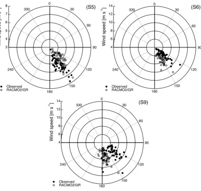
The mean wind direction along the K-transect is south-southeasterly (Fig. 7). This dominant wind direction is determined by the storms and the persistent katabatic flow that is deflected to the right of the downslope direction due to the Coriolis force. The downslope (cross-isobar) component is maintained by friction. The wind direction is

15

well simulated by RACMO2/GR, although it is too strong (26 degrees on monthly basis) deflected at S9, possibly due to a too small surface roughness length.

4.3 Humidity at 2 m

The near-surface specific humidity strongly depends on air temperature. Higher ele-vated sites have lower average specific humidity. When humidity is high, temperatures

20

(18)

TCD

4, 561–602, 2010

J. Ettema et al.

Title Page

Tables Figures

◭ ◮

Back Close

Full Screen / Esc

Interactive Discussion flux of water gas at the K-transect sites, especially the lower ones in summer. At S6,

the agreement of the daily RACMO2/GR values and observations is good (R=0.98; Fig. 8a), both for the very low values during winter (<1 g kg−1) and for the maximum values during summer (≈4 g kg−1). The monthly bias averaged over the K-transect is

−0.1 g kg−1.

5

When analyzing the 2 m relative humidity RH2 m, it appeared that in the standard post-processing of RACMO2 data, the latent heat of vaporization is used for the com-putation of the saturated vapor pressure as prescribed by the WMO (World Meteo-rological Organization), whereas sublimation/deposition takes place at freezing winter temperatures. Since the observed RH_{2 m} is derived using the latent heat of

sublima-10

tion, RACMO2/GR would significantly underestimate RH_{2 m}by−14.4 %. Therefore, we recomputed the modeled RH2 musing the daily specific humidity model values and the latent heat of sublimation, which reduced the mean daily bias to−7.2%. The observed RH_{2 m}at S6 remains close to saturation throughout the year, while RACMO2/GR shows an unexpected decrease in wintertime (Fig. 8b). Both, the summer observed and

mod-15

eled RH2 mdecrease towards the lower elevations (not shown). A possible explanation is that the katabatic wind brings colder, dry air downslope and that adiabatic compres-sion and the associated heating results in a lower summer RH downslope.

4.4 Surface energy balance

Air temperature near the surface is strongly coupled to the surface temperature T_s,

20

which is determined by the surface energy balance (SEB). The SEB (Eq. 3) over a snow/ice surface is largely controlled by the radiative fluxes, the surface albedo, and to a lesser extent by the turbulent fluxes and the subsurface heat flux (Van den Broeke et al., 2008b,a). The performance of RACMO2/GR for di_fferent terms in the SEB will be discussed in this order. Fluxes directed towards to the surface are defined as positive.

25

(19)

TCD

4, 561–602, 2010

J. Ettema et al.

Title Page

Tables Figures

◭ ◮

Back Close

Full Screen / Esc

4.4.1 Net solar radiation and surface albedo

The SEB is strongly influenced by net solar radiation that is absorbed at the surface and drives a clear seasonal and diurnal cycle unless the energy is used for melting. Along the K-transect, the model bias in SW_↓ is inconsistent. While RACMO2/GR es-timates SW_↓ to be 126 W m−2 for all three sites, the observations are less uniform.

5

A positive model bias of +14 W m−2 (11.2%) is found at S5 and a negative bias of

−10 W m−2 (7.8%) at S9. Inaccuracies in modeled clear-sky transmissivity, clouds, and/or cloud/radiation interactions in RACMO2/GR and in the ERA-40 forcings can cause these deviations from the observations. Quantification of a bias in each of these processes separately cannot be clarified without more detailed cloud-radiation

obser-10

vations and modeling.

The reflected solar radiation depends on the amount of incident solar radiation at the surface and the surface albedo. The latter is observed to be asymmetric through the year in the ablation zone (Van den Broeke et al., 2008a). Comparing daily model output with the K-transect observations reveals a too early decrease and a too late

15

increase in modeledα, by only a few days up to weeks (Fig. 9). In early summer, the winter snowpack melts, leading to a transition from a dry snow pack to a wet snow pack with α of≈0.7, followed by the surfacing of the underlying glacier ice with α of

≈0.5. The rate of this transition process is hard for the model to capture, since the modeled surface albedo is determined based on the density of the upper 5 cm of dry

20

snow, unaffected by the presence of water in the snowpack. Furthermore, in reality there is some redistribution of falling snow by the wind occurs (Van den Broeke et al., 2008a), where the radiation sensor is mounted on the AWSs that stands on top of an ice hummock (Fig. 3) and thus there is likely sampling bias toward lower albedo, especially in the early melt season.

25

(20)

TCD

4, 561–602, 2010

J. Ettema et al.

Title Page

Tables Figures

◭ ◮

Back Close

Full Screen / Esc

Interactive Discussion the robustness of the model,α responds only to significant changes in the density of

the upper 5 cm of the snow/firn/ice pack, which requires a more substantial snowfall event. The same discrepancy between model and observations is responsible for the late increase in the modelα during autumn, as fresh snow starts to cover the glacier ice at sites S5 and S6 or wet snow as in the case of the higher S9 site. Overall, the

5

surface albedo evolution through all four summers (2004–2007) is captured reasonably well (quantified below) by RACMO2/GR (R=0.73), taking into account that the ablation zone is characterized by a very inhomogeneous surface.

The underestimation of the albedo in early summer and in autumn leads, on aver-age, to a positive model bias in the reflected solar radiation of+8 W m−2averaged over

10

the K-transect (not shown). In the ablation zone, the positive biases in the reflected solar radiation lead to an overestimation in the net solar radiation, with largest biases in spring and summer months (Fig. 10b). Figure 11a shows that RACMO2/GR signifi-cantly overestimates SW_netat S6 by 31% compared to the observations. As expected the bias in SWnetis smaller for most of the dry snow zone (GC-net stations in Fig. 10a),

15

where the surface albedo remains relatively high and constant throughout the year. Only a significant deviation from the assumed fresh snowα of 0.85 may result in an overestimation at the accumulation zone sites. The correlation between net radiation observed at 20 ice sheet locations and modeled is 0.79 with climatological mean bias of 2.5 W m−2and RMSE of 3.3 W m−2.

20

4.4.2 Net longwave radiation

At S6, the daily variation in net longwave radiation LWnet is well captured by RACMO2/GR (Fig. 11b). The model tends to underestimate the lower range of val-ues during the winter months. This negative bias is caused by an underestimation of LW↓, with as largest bias 25 W m

−2

. Van de Berg et al. (2007) found a similar problem

25

(21)

TCD

4, 561–602, 2010

J. Ettema et al.

Title Page

Tables Figures

◭ ◮

Back Close

Full Screen / Esc

Interactive Discussion potential bias in cloud properties on LW_↓. At S6, the resulting winter negative bias in

LWnetis≈20 W m

−2

, since the monthly average bias in LW↑is only 5 W m −2

due to sur-face temperature bias (Fig. 12a). In summer, the LW_↑ bias diminishes as the melting surface limits the surface temperature. For S9, the performance of RACMO2/GR is similar to S6. For S5 however, the cold bias (see Fig. 4b) results in an underestimation

5

of LW_↑in winter of 25 W m−2, compensating for the bias in LW_↓(Fig. 12a).

4.4.3 Net radiation

In Fig. 11c, the net result of the daily solar and infrared radiation fluxes is presented for S6. In wintertime, solar radiation is reduced to near zero and thus LWnet drives the surface radiation budget. The negative bias in LW_↓ leads to an underestimation of

10

net radiation and is thought to be the result of underestimated clear skyLW radiance and/or of cloudiness (see Sect. 4.1). In summertime, the positive bias in SWnet is the dominant contribution to an overestimation of the net radiation absorbed at the surface. Figure 12b shows that for S6 the largest disagreement is found in spring, when the negative bias in albedo is largest. At S5 and S9, the bias in net radiation is smaller

15

due to a better representation of the surface albedo variability in the summer months. A similar bias is found for the GC-net sites JAR1 and Swiss Camp that are located in environments comparable to S9 (not shown).

4.4.4 Turbulent heat fluxes

Figure 13a shows that the daily sensible heat flux SHF at S6 is positive throughout the

20

year, which indicates that the atmosphere continuously transfers heat to the surface. The double maxima (winter and summer) correspond to the maxima in wind shear and temperature gradient between the surface and atmosphere, which are coupled through the katabatic forcing. During winter, RACMO2/GR simulates an excess in SHF of 15 W m−2 at S6 and S9 (Fig. 14a) that balances most of the surplus in net

25

(22)

TCD

4, 561–602, 2010

J. Ettema et al.

Title Page

Tables Figures

◭ ◮

Back Close

Full Screen / Esc

Interactive Discussion It is known that the mixing scheme in RACMO2 is too active, especially under very

stable atmospheric conditions (Van Meijgaard et al., 2008). This SHF winter bias is smaller at S5, because this site is closer to the ice margin and affected by a deeper katabatic wind circulation, so the modeled and observed mixing layer depth are more equivalent. Here, the excess LW cooling during winter is only partly compensated by

5

the overestimated SHF. During the summer, the largest positive bias is found at S6 (about+20 W m−2), while at S5 and S9 the bias (−4.9 and +4.1 W m−2, respectively) are much smaller.

The annual cycle of latent heat flux LHF is of importance to the SEB, with deposi-tion in winter and sublimadeposi-tion from the surface in spring and summer (Fig. 13b). To

10

obtain a realistic sublimation, it is important that at least the surface temperature is cor-rectly represented. Differences between RACMO2/GR and observational sites along the K-transect are less than 5 W m−2in winter months and 10 W m−2on average during summer (Fig. 14b). The annual bias is−2.0 W m−2averaged over these 3 sites. The largest monthly biases are found at S5. It should be noted here that “observed”

turbu-15

lent fluxes are approximated by the bulk fluxes and they are also somewhat uncertain as they may underestimate deposition (Box and Ste_ffen, 2001).

5 Summary and conclusions

An assessment of the performance of RACMO2/GR, a regional climate model with physical parameterizations optimized for use over the extensive ice sheets, is

pre-20

sented using in situ observations on and around the Greenland ice sheet. This analysis has primarily focused on the near-surface atmospheric state (temperature, humidity, wind speed and direction), and the surface energy balance components including the radiative fluxes.

We found a good correlation (R=0.97, RMSE=4.0◦C) between modeled and

mea-25

(23)

TCD

4, 561–602, 2010

J. Ettema et al.

Title Page

Tables Figures

◭ ◮

Back Close

Full Screen / Esc

Interactive Discussion found over the ice sheet/tundra. The largest monthly bias (−5◦C) occurs for winter at

the ice margin, whereas in the higher elevated ablation and in the percolation zone, the temperature evolution is captured well.

The di_fference between the modeled and measured wind speed appears to be sub-stantial at several locations, although generally the agreement is reasonable (R=0.74,

5

RMSE=1.9 m s−1). At about 60 out of the 70 stations, the difference in climatologi-cal mean 10 m wind speed is smaller than 2 m s−1. Local topographical conditions at the stations and necessarily smoothing of steep terrain in the model make it difficult to directly compare the near-surface winds with model values, especially for the land sites. The persistency of the katabatic wind circulation is captured well by the model.

10

The small deviations in wind direction in the ablation zone are probably caused by too small/large surface roughness lengths.

The surface energy balance is evaluated using SEB observations from three AWSs in the ablation and percolation zone along the K-transect and from those AWSs of the GC-net for which high-quality daily measurements were made available. The modeled

15

SW_net radiation flux matches the observations well (R=0.79) in the dry snow zone, whereas it is overestimated in the ablation and percolation zone. The model has diffi -culties in simulating the instant decrease in surface albedo due to wetting and melting of snow and the sudden increase when a thin layer of fresh snow covers the bare glacier ice. Keeping in mind that the surface in the ablation zone is very

inhomoge-20

neous, which reduces the representation of the single point observations, the model captures the changing surface conditions under melting conditions reasonably well. The found biases in the SEB components are not consistent over the K-transect

It is known that RACMO2 underestimates the downwelling longwave radiation at low atmospheric temperatures, which is related to an underestimation of the clear-sky

com-25

(24)

re-TCD

4, 561–602, 2010

J. Ettema et al.

Title Page

Tables Figures

◭ ◮

Back Close

Full Screen / Esc

Interactive Discussion gional climate models driven by analysis products with inherent cloud-radiation biases.

During winter, an excess SHF of 15 W m−2 balances most of the excess LW cooling, except for the lower ablation zone. Under extremely stable conditions, the vertical mix-ing scheme is too active, which introduces a compensatmix-ing error. As a result, only a small bias is found in the surface and 2 m temperature. The evaluation described here

5

demonstrated that RACMO2/GR is capable of simulating realistic present-day near-surface characteristics of the Greenland atmosphere on daily and monthly timescales without post-calibration or reinitialisation during the 51-year simulation.

References

Andreas, E. L.: A Theory for the Scalar Roughness and the Scalar Transfer Coefficients over

10

Snow and Sea Ice, Bound.-Lay. Meteorol., 38, 159–184, 1987. 566

Bamber, J. L., Ekholm, S., and Krabill, W. B.: A new, high resolution digital elevation model of Greenland fully validated with airborne laser data, J. Geophys. Res., 106, 33773–33780, 2001. 565, 589

Bougamont, M., Bamber, J. L., and Greuell, W.: A Surface Mass Balance Model for the

Green-15

land Ice Sheet, J. Geophys. Res., 110, F04018, doi:10.1029/2005JF000348, 2005. 567, 570

Box, J. E. and Rinke, A.: Evaluation of Greenland Ice Sheet Surface Climate in the HIRHAM Regional Climate Model Using Automatic Weather Station Data, J. Climate, 16, 1302–1319, doi:10.1175/1520-0442(2003)16, 2003. 571

20

Box, J. E. and Steffen, K.: Sublimation on the Greenland ice sheet from automated weather station observations, J. Geophys. Res., 106, 33965–33981, 2001. 582

Box, J. E., Bromwich, D. H., Veenhuis, B. A., Bai, L.-S., Stroeve, J. C., Rogers, J. C., Steffen, K., Haran, T., and Wang, S.-H.: Greenland Ice Sheet Surface Mass Balance Variability (1988– 2004) from Calibrated Polar MM5 Output, J. Climate, 19, 2783–2800, 2006. 565

25

Bromwich, D. H.: An extraordinary katabatic wind regime at Terra Nova Bay, Antarctica, Mon. Weather Rev., 117, 688–695, 1989. 576

Brutsaert, W.: Evaporation into the atmosphere, D. Reidel, 1982. 568

(25)

TCD

4, 561–602, 2010

J. Ettema et al.

Title Page

Tables Figures

◭ ◮

Back Close

Full Screen / Esc

observed climate of Greenland, 1958–1999 – with climatological standard normals 1961–90, technical report 00-18, Danish Meteorological Institute, Ministery of Transport, Copenhagen, Denmark, 2001. 573

Deardorff, J. W.: Dependence of air-sea transfer coefficients on bulk stability, J. Geophys. Res., 73, 2549–2557, 1968. 572

5

Dyer, A. J.: A review of flux-profile relationships, Bound.-Lay. Meteorol., 7, 363–372, 1974. 565 Ettema, J., van den Broeke, M. R., van Meijgaard, E., van de Berg, W. J., Bamber, J. L., Box, J. E., and Bales, R. C.: Higher surface mass balance of the Greenland ice sheet re-vealed by high-resolution climate modeling, Geophys. Res. Lett., 36, L12501, doi:10.1029/ 2009GL038110, 2009. 563

10

Ettema, J., van den Broeke, M. R., van Meijgaard, E., and van de Berg, W. J.: Climate of the Greenland ice sheet using a high-resolution climate model – Part 2: Near-surface climate and energy balance, The Cryosphere Discuss., 4, 603–639, 2010,

http://www.the-cryosphere.net/4/603/2010/. 563

Fettweis, X.: Reconstruction of the 1979–2006 Greenland ice sheet surface mass balance

15

using the regional climate model MAR, The Cryosphere, 1, 21–40, 2007, http://www.the-cryosphere-discuss.net/1/21/2007/. 565

Genthon, C.: Climate and surface mass balance of polar ice sheets in 40/15, ERA-40 Project Report Series, 2001. 566

Greuell, W. and Konzelman, T.: Numerical Modelling of the Energy Balance and the

20

Englacial Temperature of the Greenland Ice Sheet. Calculations for the ETH-Camp Loca-tion (West Greenland, 1155 m a.s.l.), Global Planet. Change, 9, 91–114, doi:10.1016/0921-8181(94)90010-8, 1994. 569

Hanna, E., Huybrechts, P., Janssens, I., Cappelen, J., Steffen, K., and Stephens, A.: Runoff

and mass balance of the Greenland Ice Sheet: 1958-2003, J. Geophys. Res., 110, D13108,

25

doi:10.1029/2004JD005641, 2005. 574

Hanna, E., Huybrechts, P., Steffen, K., Cappelen, J., Huff, R., Shuman, C., Irvine-Fynn, T., Wise, S., and Gri_ffiths, M.: Increased runo_fffrom melting from the Greenland ice sheet: a response to global warming, J. Climate, 21, 331–341, doi:10.1175/2007JCLI1964.1, 2008. 565

30

(26)

TCD

4, 561–602, 2010

J. Ettema et al.

Title Page

Tables Figures

◭ ◮

Back Close

Full Screen / Esc

Herron, M. M. and Langway, C. C.: Firn Densification: an Empirical Model, J. Glaciol., 25, 373–385, 1980. 567

Louis, J.-F.: A parametric model of vertical eddy fluzes in the atmosphere, Bound.-Lay. Meteo-rol., 17, 187–202, 1979. 565

Masson, V., Champeaux, J.-L., Chauvin, F., Meriguet, C., and Lacaze, R.: A global database of

5

land surface parameters at 1-km resolution in meteorological and climate models, J. Climate, 16, 1261–1282, 2003. 565

Oerlemans, J. and Vugts, H. F.: A Meteorological experiment in the melting zone of the Green-land ice sheet, B. Am. Meteorol. Soc., 74, 3–26, 1993. 563

Reeh, N.: Parameterization of melt rate and surface temperature on the Greenland ice sheet,

10

Polarforschung, 59(3), 113–128, 1991. 570

Reijmer, C. H., van Meijgaard, E., and van den Broeke, M. R.: Numerical Studies with a Re-gional Atmospheric Climate Model Based on Changes in the Roughness Length for Momen-tum and Heat over Antarctica, Bound.-Lay. Meteorol., 111, 313–337, 2004. 565

Reijmer, C. H., van Meijgaard, E., and van den Broeke, M. R.: Evaluation of temperature

15

and wind over Antarctica in a Regional Atmospheric Climate Model using one year of Au-tomatic Weather Station data and upper air observations, J. Geophys. Res., 110, D04103, doi:10.1029/2004JD005234, 2005. 576

Smeets, C. J. P. P. and Van den Broeke, M. R.: The parameterisation of scalar transfer over rough ice, Bound.-Lay. Meteorol., 128, 339–355, doi:10.1007/s10546-008-9290-z, 2008.

20

566

Steffen, K. and Box, J. E.: Surface climatology of the Greenland Ice sheet: Greenland Climate Network 1995-1999, J. Geophys. Res., 106, 33951–33964, 2001. 563, 571, 574, 576 Sterl, A.: On the (in)homogeneity of reanalysis products, J. Climate, 17, 3866–3873, 2004. 564 Stroeve, J., Box, J. E., Gao, F., Liang, S., Nolin, A., and Schaaf, C.: Accuracy assessment of

25

MODIS 16-day albedo product for snow: Comparison with Greenland in situ measurements, Remote Sen. Environ., 94, 46–60, 2005. 569

Und én, P., Rontu, L., J ärvinen, H., Lynch, P., Calvo, J., Cats, G., Cuxart, J., Eerola, K., Fortelius, C., Garcia-Moya, J. A., Jones, C., Lenderink, G., McDonald, A., McGrath, R., Navascues, B., WoetmanNielsen, N., Ødegaard, V., Rodriguez, E., Rummukainen, M., R õ õm, R., Sattler, K.,

30

(27)

TCD

4, 561–602, 2010

J. Ettema et al.

Title Page

Tables Figures

◭ ◮

Back Close

Full Screen / Esc

Uppala, S. M., Kallberg, P. W., Simmons, A. J., Andea, U., Bechtold, V. C. C., Fiorino, M., Gibson, J. K., Haseler, J., Hernandez, A., amd X. Li, G. A. K., Onogi, K., Saarinen, S., Sokka, N., Allan, R. P., Anderssen, E., Arpe, K., Balmaseda, M. A., Beljaars, A. C. M., van de Berg, L., Bidlot, J., Bormann, N., Caires, S., Chevallier, F., Detlof, A., Dragosavac, M., Fisher, M., Fuentes, M., Hagemann, S., Holm, E., Hoskins, B. J., Isaksen, L., Janssen, P.

5

A. E. M., Jenne, R., McNally, A. P., Mahfouf, J.-F., Morcette, J.-J., Rayner, N. A., Saunders, R. W., Simon, P., Sterl, A., Trenberth, K. E., Untch, A., Vasiljevic, D., Viterbo, P., and Woollen, J.: The ERA-40 re-analysis, Quart. J. Roy. Meteorol. Soc., 131, 2961–3012, doi:10.1256/qj. 04.176, 2005. 564

Van de Berg, W. J., van den Broeke, M. R., Reijmer, C. H., and van Meijgaard, E.:

Reassess-10

ment of the Antarctic surface mass balance using calibrated output of a regional atmospheric climate model, J. Geophys. Res., 111, D11104, doi:10.1029/2005JD006495, 2006. 563, 566 Van de Berg, W. J., van den Broeke, M. R., and van Meijgaard, E.: Heat budget of the East Antarctic lower atmosphere derived from a regional atmospheric climate model, J. Geophys. Res., 112, D23101, doi:10.1029/2007JD008613, 2007. 580

15

Van den Broeke, M., Smeets, P., Ettema, J., and Kuipers Munnike, P.: Surface radiation balance in the ablation zone of the west Greenland ice sheet, J. Geophys. Res., 113, D13105, doi: 10.1029/2007JD009283, 2008a. 571, 572, 578, 579

Van den Broeke, M., Smeets, P., Ettema, J., van der Veen, C., van de Wal, R., and Oerlemans, J.: Partitioning of melt energy and meltwater fluxes in the ablation zone of the west Greenland

20

ice sheet, The Cryosphere, 2, 179–189, 2008,

http://www.the-cryosphere-discuss.net/2/179/2008/.b. 571, 572, 578

Van den Broeke, M. R.: Characteristics of the lower ablation zone of the West Greenland ice sheet for energy-balance modelling, Ann. Glaciol., 23, 160–166, 1996. 572

Van den Broeke, M. R., Duynkerke, P. G., and Oerlemans, J.: The observed katabatic flow

25

at the edge of the Greenland ice sheet during GIMEX-91, Global Planet. Change, 9, 3–15, 1994. 575

Van den Broeke, M. R., Smeets, P., and Ettema, J.: Surface layer climate and turbulent ex-change in the ablation zone of the west Greenland ice sheet, Int. J. Climatol., 2309–2323, doi:10.1002/joc.1815, 2008c. 572, 577

30

(28)

TCD

4, 561–602, 2010

J. Ettema et al.

Title Page

Tables Figures

◭ ◮

Back Close

Full Screen / Esc

Van Lipzig, N. P. M., van Meijgaard, E., and Oerlemans, J.: Evaluation of a Regional Atmo-spheric Model Using Measurements of Surface Heat Exchange Processes from a Site in Antarctica, Mon. Weather Rev., 127, 1994–2011, 1999. 563

Van Meijgaard, E., van Ulft, L. H., van de Berg, W. J., Bosveld, F. C., van den Hurk, B. J. J. M., Lenderink, G., and Siebesma, A. P.: The KNMI regional atmospheric climate model RACMO

5

version 2.1, Tech. Rep. 302, KNMI, P.O. box 201, 3730 AE, De Bilt,the Netherlands, 2008. 563, 565, 582

White, P. W., ed.: IFS documentation CY23r4: Part IV physical processes, online available at: http://www.ecmwf.int/research/ifsdocs/, 2004. 564

Yang, D., Kane, D., Zhang, Z., Legates, D., and Goodison, B.: Bias corrections of long-term

10

(29)

TCD

4, 561–602, 2010

J. Ettema et al.

Title Page

Tables Figures

◭ ◮

Back Close

Full Screen / Esc

Fig. 1. Map of Greenland featuring the model domain, relaxation borders (the outer 16 grid

(30)

TCD

4, 561–602, 2010

J. Ettema et al.

Title Page

Tables Figures

◭ ◮

Back Close

Full Screen / Esc

Fig. 2.Schematic representation of modeled processes that determine surface mass balance.

(31)

TCD

4, 561–602, 2010

J. Ettema et al.

Title Page

Tables Figures

◭ ◮

Back Close

Full Screen / Esc

Fig. 3. Images of the AWSs along the K-transect and their surroundings at S5, S6 and S9.

(32)

TCD

4, 561–602, 2010

J. Ettema et al.

Title Page

Tables Figures

◭ ◮

Back Close

Full Screen / Esc

-35 -30 -25 -20 -15 -10 -5 0 5

GC net DMI K-transect

Modelled 2 m temperature [

o C]

Observed 2 m temperature [oC] (a)

-6 -5 -4 -3 -2 -1 0 1 2 3

1 2 3 4 5 6 7 8 9 10 11 12

S5 S6 S9

2 m temperature [

o C]

month (b)

Fig. 4. Model performance for 2 m temperature [◦C]. (a)model versus observations for

(33)

TCD

4, 561–602, 2010

J. Ettema et al.

Title Page

Tables Figures

◭ ◮

Back Close

Full Screen / Esc

-40 -30 -20 -10 0 10

Jan/1 Feb/1 Mar/1 Apr/1 May/1 Jun/1 Jul/1 Aug/1 Sep/1 Oct/1 Nov/1 Dec/1 Jan/1

2 m temperature [

oC]

Date (a)

0 5 10 15 20

Wind speed [m s

-1]

Date

(b)

0.65 0.7 0.75 0.8 0.85 0.9 0.95 1

2004/1 2004/7 2005/1 2005/7 2006/1 2006/7 2007/1 2007/7

Directional constancy [-]

Date (c)

Fig. 5. Comparison of simulated (gray lines) and observed (black lines) daily averaged (a)

2 m temperature [◦C],(b)daily mean 10 m wind speed [m s−1] at S6 for the year 2004, and(c)

(34)

TCD

4, 561–602, 2010

J. Ettema et al.

Title Page

Tables Figures

◭ ◮

Back Close

Full Screen / Esc

0 2 4 6 8 10

GC net DMI K-transect

Modelled 10 m wind speed [m s

-1 ]

Observed 10 m wind speed [m s-1]

(a)

-3 -2 -1 0 1 2

1 2 3 4 5 6 7 8 9 10 11 12

S5 S6 S9

10 meter wind speed [m s

-1 ]

month (b)

Fig. 6. Model performance for 10 m wind speed [m s−1]. (a) model versus observations for

(35)

TCD

4, 561–602, 2010

J. Ettema et al.

Title Page Abstract Introduction Conclusions References Tables Figures ◭ ◮ ◭ ◮ Back Close

Full Screen / Esc

Printer-friendly Version Interactive Discussion 3 4 5 6 7 8 0 30 60 90 120 150 180 210 240 330 Observed RACMO2/GR

Wind speed [m s

-1] (S5)

4 6 8 10 12 14 0 30 60 90 120 150 180 210 240 330 Observed RACMO2/GR

Wind speed [m s

-1] (S6)

4 6 8 10 12 14 0 30 60 90 120 150 180 210 240 330 Observed RACMO2/GR

Wind speed [m s

-1 ] (S9)

Fig. 7.Comparison of simulated (open circles) and observed (solid circles) monthly averaged

(36)

TCD

4, 561–602, 2010

J. Ettema et al.

Title Page

Tables Figures

◭ ◮

Back Close

Full Screen / Esc

0 1 2 3 4 5

Specific humidity [g kg

-1 ]

Date (a)

40 50 60 70 80 90 100

Relative humidity [%]

Date

(b)

Fig. 8.Comparison of simulated (gray lines) and observed (black lines) daily averaged 2 m(a)

(37)

TCD

4, 561–602, 2010

J. Ettema et al.

Title Page

Tables Figures

◭ ◮

Back Close

Full Screen / Esc

0.4 0.5 0.6 0.7 0.8 0.9 1

Apr/1 May/1 Jun/1 Jul/1 Aug/1 Sep/1 Oct/1

Albedo [-]

Date (S5)

0.4 0.5 0.6 0.7 0.8 0.9 1

Albedo [-]

Date (S6)

0.4 0.5 0.6 0.7 0.8 0.9 1

Albedo [-]

Date (S9)

Fig. 9.Time evolution of the daily surface albedo [−] in the observations (black lines) and model

(38)

TCD

4, 561–602, 2010

J. Ettema et al.

Title Page

Tables Figures

◭ ◮

Back Close

Full Screen / Esc

10 15 20 25 30 35 40 45 50

K-transect GC net

Modelled net solar radiation [W m

-2 ]

Observed net solar radiation [W m-2] (a)

-20 -10 0 10 20 30 40 50 60

1 2 3 4 5 6 7 8 9 10 11 12

S5

S6 S9

Net solar radiation [W m

-2 ]

month (b)

Fig. 10. Model performance for surface net solar radiation [W m−2](a)model versus

observa-tions for GC-net (black) and K-transect (green) averaged over the available measuring period,

(39)

TCD

4, 561–602, 2010

J. Ettema et al.

Title Page

Tables Figures

◭ ◮

Back Close

Full Screen / Esc

Interactive Discussion 0

50 100 150 200

SW

net

[W m

-2]

Date (a)

-100 -80 -60 -40 -20 0 20

LW

net

[W m

-2]

Date (b)

-100 -50 0 50 100 150

Net radiation [W m

-2]

Date (c)

Fig. 11.Comparison of simulated (gray lines) and observed (black lines) daily averaged values