INTRODUCTION
The evaluation of genotypes in crosses is a com-mon practice in plant breeding. In maize (Zea mays L.), after Jones (1918) suggested the use of double crosses for commercial use, the evaluation of the genetic potential of inbred lines to be used in hybrids was based on all pos-sible combinations among them (Hallauer and Miranda Filho, 1995). The use of the top-cross procedure (Davis, 1927; Jenkins and Brunson, 1932) allowed the evaluation of a greater number of lines in crosses with a common tester. Sprague and Tatum (1942) introduced the concept of general combining ability (GCA) and specific combin-ing ability (SCA) when genotypes are crossed in all pos-sible combinations (diallel cross). In this sense, the top-cross procedure allows the estimation of combining abil-ity with the tester, but no information is provided on SCA for specific crosses among the set of lines (genotypes). In addition, the combining ability effect of a line is not a prop-erty of the line alone but rather depends on the set of lines to which it has been crossed (Kempthorne and Curnow, 1961). Therefore, the general combining ability of a line in a diallel mating scheme should not be necessarily the same as its combining ability in a cross with a common tester (top-cross).
The diallel mating scheme is still used in plant breeding and several methodologies are available (Singh
and Chaudhary, 1979). Griffing (1956) provided four meth-ods, specified according to the nature of entries in the di-allel table, under two models (fixed and random) for the analysis of variance and estimation of GCA and SCA in diallel tables. The constraint of the diallel scheme is the number of crosses for a given set of genotypes, i.e., for n lines there will be n(n - 1)/2 crosses. Therefore, the com-plete diallel cross is feasible only for a relatively small num-ber of genotypes or lines.
Kempthorne and Curnow (1961) suggested the par-tial diallel cross to allow the evaluation of a greater num-ber of inbred lines in crosses. According to this proce-dure, each of the n lines in the set are crossed with s other lines of the same set, instead of (n - 1) lines as in the com-plete diallel. Thus, there will be ns/2 crosses in the whole set, where s ≥ 2. It is clear that n and s cannot both be odd. Crosses are made in such a way that all lines are involved in the sample of crosses. Sampling of lines is based on a reference number, k = (n + 1 - s)/2, so that the crosses are: [1 x (k + 1)], [1 x (k + 2)], ..., [1 x (k + s)]; [2 x (k + 2], [2 x (k + 3)], ..., [2 x (k + s + 1)], and so on. The lines are numbered at random.
In the partial diallel table, the model for the mean (over r replications) of the cross between lines i and i’ is Yii’= m + gi + gi’ + sii’+ eii’, where m is the the overall mean, gi is the GCA effect, sii’ is the SCA effect and eii’is the error of the cross mean.
The partial diallel cross, as proposed by Kempthorne and Curnow (1961), assumes a random sample of lines (genotypes) from one population. In addition to the estima-tion of general and specific combining ability, the partial diallel cross analysis of variance permits the estimation of variance components at the intrapopulation level.
THE PARTIAL CIRCULANT DIALLEL CROSS AT THE INTERPOPULATION LEVEL
José B. Miranda Filho and Roland Vencovsky
A
BSTRACTThe partial circulant diallel cross mating scheme of Kempthorne and Curnow (Biometrics 17: 229-250, 1961) was adapted for the evaluation of genotypes in crosses at the interpopulation level. Considering a random sample of n lines from base population I, and that each line is crossed with s lines from opposite population II, there will be ns sampled crosses that are evaluated experimentally. The means of the ns sampled crosses and the remaining n(n - s) crosses can be predicted by the reduced model Yij= m + gi+ gj, where Yij is the mean of the cross between line i (i = 1,2,...,n) of population I and line j (j = 1’,2’,...,n’) of population II; µ is the general mean, and gi and gj refer to general combining ability effects of lines from populations I and II, respectively. Specific combining ability (sij) is estimated by the difference (sij = Yij - m - gi- gj). The sequence of crosses for each line (i) is [i x j], [i x (j + 1)], [i x (j + 2)], ..., [i x (j + s -1)], starting with i = j = 1 for convenience. Any j + s -1 > n is reduced by subtracting n. A prediction procedure is suggested by changing gi and gj by the contrasts τi = Yi. - Y.. and τj = Y.j - Y..; the correlation coefficient (r) was used to compare the efficiency of g’s and τ’s for selection of lines and crosses. The analysis of variance is performed with the complete model Yij= µ + gi+ gj + sij+ eij, and the sum of squares due to general combining ability is considered for each population separately. An alternative analysis of variance is proposed for estimation of the variance components at the interpopulation level. An analysis of ear length of maize in a partial diallel cross with n = 10 and s = 3 was used for illustration. For the 30 interpopulation crosses analyzed the coefficient of determination (R2), involving observed and estimated hybrid means, was high for the reduced (g) model [R2 (Y
ij, Yij) = 0.960] and smaller for the simplified (τ) model [R2 (Yij, Yij) = 0.889]. Results indicated that the proposed procedure may furnish reliable estimates of means of hybrids not available in the partial diallel.
^ ^ ^ ^
^ ^ ^ ^
^ ^
^ ^
In modern maize breeding, it is a common proce-dure to cross lines from two sources (populations) in an attempt to maximize the genetic effects, including hetero-sis, in the hybrid cross (Hallauer and Miranda Filho, 1995). Therefore, for n lines from each source there would be n² possible crosses; although n²is smaller than 2n(2n - 1)/2 (all possible crosses among 2n lines), there is still a large number of crosses when 2n is large. Such a scheme should be useful for evaluation of crosses between two fixed sets of lines or varieties (Geraldi and Miranda Filho, 1988) but the method is not feasible for a greater number (e.g., n = 100) of lines from each source. In the present study we propose an adaptation of the circulant partial diallel cross of Kempthorne and Curnow (1961) for the evaluation of inbred lines in crosses at the interpopulation level.
MATERIAL AND METHODS
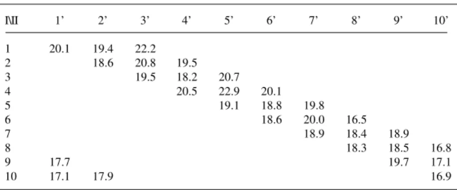
We consider two sets of n lines or genotypes, rep-resenting two groups or populations (I and II). The lines must be random samples of the respective populations of lines and the crosses are arranged in such a way that all lines enter in the cross schedule. Each line of population-I is crossed with s lines of population-population-Ipopulation-I, and vice-versa, so that there will be ns sampled crosses out of n² possible crosses. The cross arrangement is an adaptation of the par-tial diallel of Kempthorne and Curnow (1961). The se-quence of crosses of a line (i) is: i x j; i x (j + 1); i x (j + 2); ...; i x (j + s - 1). An example is given for n = 10 and s = 3, where data refer to ear length (cm) in crosses between lines from two maize populations (SUWAN and ESALQ-PB1) evaluated in experiments conducted at Piracicaba, SP (Table I).
The model for each cross mean is:
Yij = m + gi + gj + sij + eij
where m is the overall mean; gi and gj are the GCA effects of lines from populations I and II, respectively; sij is the
SCA effect, and eij is the experimental error associated with the hybrid mean.
The pertinent analysis of variance and estimation of effects in the model is done following the least square procedure, according to the matrix equation: Y = Xβββββ +εεεεε, where Y is the vector of observed means (ns sampled crosses), X is the matrix of coefficients, βββββ is the vector of parameters and εεεεε is the vector representing the experimental error.
For both the analysis of variance and estimation of effects we considered the reduced model Yij = m + gi + gj + δij, so that δ also includes the sij effects as deviations from the reduced model. Because X is a singular matrix, the fol-lowing restrictions must be imposed for solution:
∑ gi = ∑ gj = 0.
RESULTS AND DISCUSSION
Analysis of variance
For the analysis of variance and estimation of effects, the ordinary least square procedure was used. Parameters in the reduced model (mean and combining ability effects) are estimated by solving normal equations [βββββ = (X’X)-1 X’Y] derived from Yij= m + gi + gj + δ1ij.
The sums of squares for parameters in the com-plete model (Model 1) and reduced models are represented as shown in Table II.
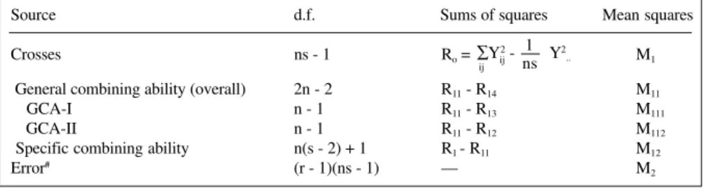
The estimates of GCA effects (gi, gj) can also be obtained from the reduced model (Model 1) and the SCA (sij) is obtained by the differences from the observed means which are explained by the complete model. For obtaining the standard errors of the estimates, appropriate programs of statistical analysis can be used. The sums of squares due to variation among crosses is partitioned into general and specific combining ability according to the complete model (Table III).
Table I - Means (over three replications) of ear length (cm) of thirty single cross
maize hybrids in a partial diallel scheme.
I\II 1’ 2’ 3’ 4’ 5’ 6’ 7’ 8’ 9’ 10’
1 20.1 19.4 22.2
2 18.6 20.8 19.5
3 19.5 18.2 20.7
4 20.5 22.9 20.1
5 19.1 18.8 19.8
6 18.6 20.0 16.5
7 18.9 18.4 18.9
8 18.3 18.5 16.8
9 17.7 19.7 17.1
10 17.1 17.9 16.9
I - SUWAN; II - ESALQ-PB1.
Model (1)
^ ^
j i
The expected values of mean squares in the analy-sis of variance shown in Table II are not available, so that unbiased estimates of the variance components are not pos-sible from Table II. A relative measure of effectiveness is the coefficient of determination (R²), which is the square of the correlation between observed and predicted means. It also measures the ratio between the sum of squares due to the reduced model and the total sum of squares (com-plete model). However, R2 is not always realistic due to the difference between the number of degrees of freedom (d.f.) for GCA and SCA. For s = 2, d.f. = 1 for SCA for
any value of n and, consequently, R2≈ 1. For s > 2, d.f. for SCA is about (s - 2)/2 times d.f. for GCA, and they are approximately equal for s = 4. Therefore, for s = 4 the coefficient of determination should give a fairly good mea-sure of efficiency of the reduced model. Obviously, for a given n and s, R² tends to be higher for small or nonsig-nificant SCA effects. Consequently, since SCA is due to non-additive effects, R² will be higher for traits affected primarily by additive effects.
For the diagonals in Table I, it is apparent that there is a genetic covariance between diagonal elements; the co-variance between each pair is a linear function of the vari-ance due to general combining ability (σ²). There are two variances for GCA, one for each population. For GCA-I, the covariances between diagonals are obtained directly from the scheme shown in Table I. For GCA-II, the diago-nals must be rearranged. For n = 10 and s = 3 the diagodiago-nals for obtaining the covariances are as shown in Table IV.
The two groups of diagonals (Table IV) can be ana-lyzed as two-way tables, according to the factorial model
(Model 2):
Yik= m + τi + δk + (τδ)ik + eik for group I, and Yjk= m + τj + δk + (τδ)jk + ejk for group II,
Table IV - Schematic presentation of the diagonals of Table I rearranged according to
the source population (I and II).
Lines I D1 D2 D3 Lines II D1’ D2’ D3’
1 1 x 1’ 1 x 2’ 1 x 3’ 1’ 1’ x 1 1’ x 1.0’ 1’ x 9 2 2 x 2’ 2 x 3’ 2 x 4’ 2’ 2’ x 2 2’ x 1 2’ x 1.0’
3 3 x 3’ 3 x 4’ 3 x 5’ 3’ 3’ x 3 3’ x 2 3’ x 1 4 4 x 4’ 4 x 5’ 4 x 6’ 4’ 4’ x 4 4’ x 3 4’ x 2 5 5 x 5’ 5 x 6’ 5 x 7’ 5’ 5’ x 5 5’ x 4 5’ x 3 6 6 x 6’ 6 x 7’ 6 x 8’ 6’ 6’ x 6 6’ x 5 6’ x 4 7 7 x 7’ 7 x 8’ 7 x 9’ 7’ 7’ x 7 7’ x 6 7’ x 5 8 8 x 8’ 8 x 9’ 8 x 1.0’ 8’ 8’ x 8 8’ x 7 8’ x 6 9 9 x 9’ 9 x 1.0’ 9 x 1’ 9’ 9’ x 9 9’ x 8 9’ x 7 10 10 x 1.0’ 10 x 1’ 10 x 2’ 10’ 10’ x 1.0’ 10’ x 9 10’ x 8 I, II: Lines from populations I and II that are common to all diagonals of the respective group. D and D’ are diagonals representing crosses arranged for lines 1, 2, ..., 10 of population I and for lines 1', 2', ..., 10' of population II.
Table III - Analysis of variance for crosses in the partial circulant diallel scheme at the interpopulation level.
Source d.f. Sums of squares Mean squares
Crosses ns - 1 Ro= M1
General combining ability (overall) 2n - 2 R11 - R14 M11
GCA-I n - 1 R11 - R13 M111
GCA-II n - 1 R11 - R12 M112
Specific combining ability n(s - 2) + 1 R1- R11 M12
Error# (r - 1)(ns - 1) — M
2
# For a completely randomized block design.
∑Y2 - Y2 ..
1 ns
ij ij
Table II - Representation of the complete and reduced models
and their sums of squares.
Sums of squaresψ Model 1 Yij= m + gi + gj + sij + eij R1 = ∑Y2 - Y2../ns
Model 11 Yij= m + gi + gj + δ1ij R11 = R(m, gi , gj)
Model 12 Yij= m + gi + δ2ij R12 = R(m, gi)
Model 13 Yij= m + gj + δ3ij R13 = R(m, gj)
Model 14 Yij = m + δ4ij R14 = R(m) ψR = β (X’Y) for each model.
ij ij
g
where m is the overall mean and is common for both groups; τi and τj are the constant effects of the parental lines; δk is the random effects due to differences among diagonals, and (τδ)ik and (τδ)jk are interaction effects of lines with diagonals within the respective groups. The last effect is the error term in both models.
Within each group the diagonals are represented by crosses involving the same lines, so that the diagonal means differ only for the average error and for a small quantity represented by the average of the random sample of SCA effects ( ∑sij or ∑sij). The expected values of the squared effects are: E(δ²) = σ2, E(τ²) = σ² = σ², E(τ²) = σ² = σ² , and E(e2 ) = E(e2 ) = σ². Components σ² and σ² are related to the genetic interpretation of the effects, i.e., they represent the variances due to GCA of lines within groups; σ² is the variance due to SCA and σ² is the error variance adjusted for analysis involving means over r rep-lications.
The analysis of variance of the two-way tables is as shown in Table IV. The analysis for group I and for group II has a similar structure. In the expected value of mean squares, the average variance within diagonals and the error variance are the same for both groups.
The partition of the sum of squares is orthogonal within groups but non-orthogonal between groups (Table V). Because the estimates of the variance components are based on both analyses, the estimates are correlated to some extent. In this sense, we recognize that the properties of the estimators must be better known.
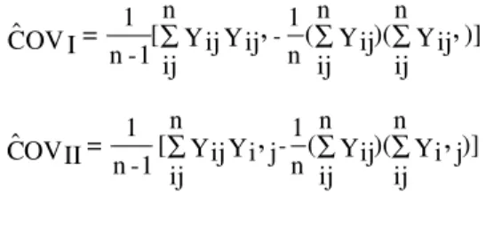
The covariance between any two diagonals is esti-mated by:
In terms of expectation the covariances are:
COVI = E [(Yij- µ)(Yij’- µ)] = E[(gi+ gj+ sij+ eij) (gi+ gj’+ sij’+ eij’)] = σ²gI
COVII = E[(Yij- µ)(Yi’j- µ)] = E[(gi + gj + sij+ eij) (gi’+ gj+ si’j+ ei’j) = σ²gII
Taking all the covariances between diagonals, there will be s(s-1)/2 estimates of σ² for each population, and the average estimate of the covariances is an average esti-mate of the variance due to GCA. The estiesti-mates of the variance components are obtained by:
COVI = COVgI = σ2 = (M
t - Mtd), in the analysis of group I, and
COVII = COVgII = σ2 = (M
t - Mtd), in the analysis of group II
σ2 = M
td + Mt- Me, and σ 2 = M
e
where σ2 stands for the variance due to combining ability of lines of the respective group, and σ2
= σ2 + σ2 + σ2 is the variance among crosses within diagonals. The latter shows the variance component due to SCA (σ²), which is estimated by
σ2 = σ2 - σ2 - σ2
It is clear that for obtaining the overall estimates, the analysis of variance shown in Table IV must be per-formed for both groups of diagonals. The estimates of the variance components (σ2 , σ2 , σ2 ) are based on Model 1 and therefore the corresponding parameters are the same as those defined for the analysis of variance in Table V.
The translation of the variance components into genetic variances is given by the functions:
σ2 = σ2 ; σ2 = σ2
; σ2 = ( )2 σ2 and
σ2
= (σ2
+ σ2
) + ( )2σ2
= σ2
+
+ ( )2σ2
where F is the coefficient of inbreeding of the lines from both non-inbred reference populations (Hallauer and Miranda Filho, 1995), assuming the same F in both sets of lines. For different inbreeding levels (FI ≠ FII), pertinent adaptations must be introduced in the above formulas.
k d i τI gI j
τII gII ik jk gI gII
s
Table V - Analysis of variance of two-way tables representing
s diagonals of group I.
Source d.f. MS
Diagonals(D) s - 1 Md σ² + σ²δ
Lines(L) n - 1 Mt σ² + σ²τδΙ+ σ²τΙ= σ² + + (σ²H - COVgI ) + sCOVgI
L x D (n - 1)(s - 1) Mtd σ² + σ²τδΙ= σ² + (σ²H - COVgI)
Error (r - 1)(ns - 1) Me σ²
Hybrids/D s(n - 1) MH/D σ² + σ²H
σ²H: Average of s variances within diagonals; COVgI : average of s(s - 1)/2
covariances between diagonals.
1 n
1 n
g
H gI gII s
s
H gI gII
s ^ ^ ^ gI 1 s ^ gII 1 s ^ H 1 s ^
gI gII s s - 1
s
gI A12
1 + F
4 A21
gII s
1 + F
2 D12
1 + F 4
H 1 + F
4 A12 A21
1 + F
2 D12 A12
1 + F
2 D12
1 + F 2 j i )] Yij n ij )( Yij n ij ( n 1 -Yij Yij n ij [ 1 -n 1 = OV
Cˆ I ∑
,
∑ ∑,
)] Y ji n ij )( Yij n ij ( n 1 -Y ji Yij n ij [ 1 -n 1 = OV
Cˆ II ∑
,
∑ ∑,
The genetic variance components are readily esti-mated by:
σ2
= (σ2 + σ2 ), and σ2 = ( )2 σ2
Estimation of cross means
The mean of sampled crosses in the diallel table can be estimated by: 1) the observed mean of the given cross in the experiment, and 2) ignoring SCA and then estimating the mean based on the reduced model: Yij = µ + gi + gj
(Model 3). The mean of the unsampled crosses can only
be estimated through (2) (Kempthorne and Curnow, 1961). Finally, for random samples of lines from two populations, the following quantities are taken into account: n: number of lines randomly sampled from each
population;
n2: number of possible crosses; s: number of crosses for each line;
ns: number of observed means of the sampled crosses, and
n(n-s): number of predicted means of the unsampled crosses.
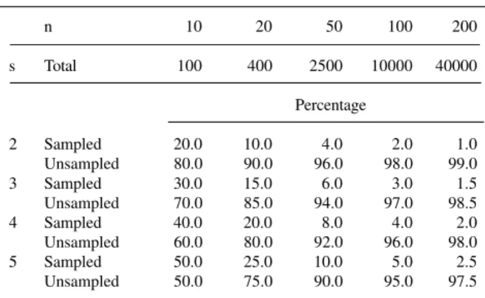
The number of sampled and unsampled crosses for several values of n and s is shown in Table VI.
A third method (3) for estimating the mean of spe-cific crosses is through Yij = m + τi + τj where τi and τj are contrasts (random effects) obtained by:
τi = Yi.- Y.. and τj = Y.j - Y..
so that ∑ τi = ∑ τj = 0. Their standard errors can be easily estimated by the square root of V(τi) = V(τj) = σ2 where σ² is the variance due to the experimental error
ad-justed for means over r replications. If the estimates ob-tained by (3) do not depart very far from those obtained by (2), or if the rank of the estimates does not change greatly, the use of (3) should be advantageous in the sense that the estimates can be obtained easily without the need of a spe-cific computer program. In practical breeding programs, where facilities of this sort are not always available, con-clusions and decisions could be faster by method (3).
In terms of model (1), for s = 3, it can be shown that:
τi = gi+ (gj + gj’ + gj”) + ∑sij + ∑eij and
τj = gj + (gi + gi’ + gi”) + ∑sij + ∑eij
It is apparent that the differences between gi and τi and between gj and τj tend to decrease for larger values of s (number of crosses of each line); consequently, the cor-relation between them tends to increase for increasing s.
Example: analysis of ear length in maize
The analysis of data (Table I) taken for illustration led to the results shown in Table VII.
The analysis shows that a significant variation was detected for GCA effects in both populations and that the amount of genetic variability does not differ greatly
be-gI gII D12 s
A12 1 + F 2
1 + F 2
^ ^ ^ ^ ^
^ ^ ^
Table VII - Analysis of variance according to the partial
circulant diallel model.
Source d.f. M.S. F
Hybrids 29 2.3005 5.80**
GCA/Populations 18 3.4125 7.10**
GCA-I 9 2.1730 4.52**
GCA-II 9 2.4456 5.09**
SCA 11 0.4809 1.21
Error 58 0.3968
** Significance level: P < 0.01.
Table VI - Total number and percentage of sampled and unsampled
crosses for some value of n (number of lines) and s (number of crosses for each line).
n 10 20 50 100 200
s Total 100 400 2500 10000 40000
Percentage
2 Sampled 20.0 10.0 4.0 2.0 1.0
Unsampled 80.0 90.0 96.0 98.0 99.0
3 Sampled 30.0 15.0 6.0 3.0 1.5
Unsampled 70.0 85.0 94.0 97.0 98.5
4 Sampled 40.0 20.0 8.0 4.0 2.0
Unsampled 60.0 80.0 92.0 96.0 98.0
5 Sampled 50.0 25.0 10.0 5.0 2.5
Unsampled 50.0 75.0 90.0 95.0 97.5
^ ^ ^ ^ ^ ^
^ ^
i j
^ ^
n - 1 ns
^ ^
1
s 1s j 1s j
1
s 1s 1s
i i
^
^
Table VIII - Analysis of variance with partition of the total sum of squares
according to the factorial model. Ear length of 30 corn hybrids.
Source d.f. MS I MS II Estimates
Hybrids 29 2.30052 2.30052 σ²gI = 0.9556
Diagonals (D) 2 0.03700 0.03700 σ²gII= 1.0919
Lines (L) 9 4.37944 4.65204 σ²S = 0.0238
L x D 18 1.51256 1.37626 σ²A12 = 2.0476
Error 58 0.39680 0.39680 σ²D12 = 0.0238
Hybrids/Diagonals 27 2.46819 2.46819
^
^ ^
^
tween populations. Specific combining ability was small and non-significant.
The analysis of variance of sets of diagonals for groups I and II, according to the two-way factorial model, is shown in Table VIII.
Although the sample of data is too small to esti-mate genetic parameters, the results are coherent with in-formation from the literature for ear length. The interpopu-lation additive genetic variance is within the range reported by Hallauer and Miranda Filho (1995) for estimates within (intra) populations. The dominance variance is very small, suggesting that ear length of maize is primarily due to ad-ditive effects. The estimates of effects (g and τ) for both populations are listed in Table IX. The degree of agree-ment between g and τ is given by the correlation coeffi-cient (r), which showed a fairly good agreement between the information based on g and τ for both populations. It is
seen that the three lines with highest values do not change when considering g or τ, for both populations. It is clear that the degree of confidence of that relation would be best determined for larger samples of lines.
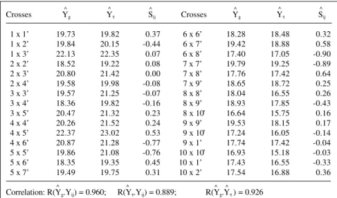
The predicted means of specific crosses were based on the two reduced models differing by their estimators of the combining ability effects namely: i) based on gi and gj , and ii) based on τi and τj. The predicted means are shown in Table X.
The correlation between the predicted means based on gi and gj and the observed means showed the high effi-ciency of the reduced model for prediction purposes. A lower correlation (0.889) was observed for prediction based on τ effects. Nevertheless, the high correlation between predictions based on g’s and τ’s indicates that the latter can be nearly as efficient as the former for the identifica-tion of desirable crosses for ear length.
Table IX - Estimates of the mean (m), GCA (gi, gj) and line combining ability (τi , τj)
effects for crosses between two maize populations.
SUWAN gi Rank τi Rank ESALQ-PB1 gj Rank τj Rank
1 2.069 (1) 1.517 (2) 1’ -1.387 (9) -0.750 (8)
2 0.743 (3) 0.583 (3) 2’ -1.276 (8) -0.417 (7)
3 -0.484 (6) 0.417 (4) 3’ 1.008 (3) 1.783 (2)
4 1.419 (2) 2.117 (1) 4’ -0.209 (6) 0.350 (4)
5 -1.097 (9) 0.183 (5) 5’ 1.904 (1) 1.850 (1)
6 -1.167 (10) -0.683 (7) 6’ 0.398 (5) 0.117 (5)
7 -0.801 (8) -0.317 (6) 7’ 1.538 (2) 0.517 (3)
8 -0.525 (7) -1.183 (9) 8’ -0.486 (7) -1.317 (9)
9 0.076 (4) -0.883 (8) 9’ 0.400 (4) -0.017 (6)
10 -0.232 (5) -1.750 (10) 10’ -1.889 (10) -2.117 (10)
Mean: M = 19.04 Correlation r(gi, τi) = 0.693 r(gj, τj) = 0.857
^ ^ ^ ^
^ ^ ^ ^
^ ^
^ ^ ^ ^ ^ ^
^ ^ ^ ^
^ ^
Table X - Estimates of specific combining ability effects (sij) and predicted means of
sampled single crosses based on two models#.
Crosses Yg Yτ Sij Crosses Yg Yτ Sij
1 x 1’ 19.73 19.82 0.37 6 x 6’ 18.28 18.48 0.32
1 x 2’ 19.84 20.15 -0.44 6 x 7’ 19.42 18.88 0.58
1 x 3’ 22.13 22.35 0.07 6 x 8’ 17.40 17.05 -0.90
2 x 2’ 18.52 19.22 0.08 7 x 7’ 19.79 19.25 -0.89
2 x 3’ 20.80 21.42 0.00 7 x 8’ 17.76 17.42 0.64
2 x 4’ 19.58 19.98 -0.08 7 x 9’ 18.65 18.72 0.25
3 x 3’ 19.57 21.25 -0.07 8 x 8’ 18.04 16.55 0.26
3 x 4’ 18.36 19.82 -0.16 8 x 9’ 18.93 17.85 -0.43 3 x 5’ 20.47 21.32 0.23 8 x 1.0’ 16.64 15.75 0.16
4 x 4’ 20.26 21.52 0.24 9 x 9’ 19.53 18.15 0.17
4 x 5’ 22.37 23.02 0.53 9 x 1.0’ 17.24 16.05 -0.14 4 x 6’ 20.87 21.28 -0.77 9 x 1’ 17.74 17.42 -0.04 5 x 5’ 19.86 21.08 -0.76 10 x 1.0’ 16.93 15.18 -0.03 5 x 6’ 18.35 19.35 0.45 10 x 1’ 17.43 16.55 -0.33
5 x 7’ 19.49 19.75 0.31 10 x 2’ 17.54 16.88 0.36
Correlation: R(Yg.Yij) = 0.960; R(Yτ.Yij) = 0.889; R(Yg.Yτ ) = 0.926 # Model 1 for Y
The correlations between g’s and τ’s (Table IX) are much smaller than the correlation between the respec-tive predicted means, indicating that selection based on τ’s is less effective among lines than among crosses, when compared with selection based on g’s. The trait (ear length) and the sample of crosses were used herein merely to il-lustrate the proposed procedure and the results were not interpreted as conclusive.
The partial circulant diallel cross at the interpopu-lation level, as proposed in this study, seems to be an alter-native method for the evaluation of the genetic value of lines or genotypes in crosses at the interpopulation level. It seems to be advantageous over other methods when the following points are considered:
1. It allows the evaluation of a greater number of lines rela-tive to the complete diallel; this point was also empha-sized by Kempthorne and Curnow (1961) for the intrapo-pulation partial diallel.
2. The number of sampled crosses (ns) allows the prediction of n(n - s) single crosses and the selection pressure on crosses is greatly increased. For example, for n = 100 and s = 3, the selection of the 10 best crosses represents a selection intensity of 0.1% .
3. The base populations are chosen on the basis of their complementary gene structure, so that the population cross combines alleles existing separately in the parents. The heterosis of the population cross is explored in the crosses between lines of divergent populations. 4. The tester of lines of each population is a sample of lines
of the opposite population, so that the combining ability effects realistically reflect the potential of lines to be used in crosses. In this sense, the topcross procedure should give less realistic information on the combining ability of lines, unless the same base populations are used as testers of each other.
5. Information is also obtained on SCA of the sampled crosses. Hypotheses about its variation can be tested in the analysis of variance and desirable specific effects can be eventually detected.
More experimental results and theoretical consid-erations of the proposed methodology will be necessary for a better understanding of its properties and its poten-tial for prediction and selection. Special attention must be given to comparisons with other methods. Of special interest will be a comparison between results obtained here and the BLUP predictions proposed by Bernardo (1994).
ACKNOWLEDGMENTS
We gratefully acknowledge Dr. Cássio R.M. Godoy (Departamento de Matemática e Estatística, ESALQ/USP) for his assistance in the statistical model and analysis, and Dr. Ana C. Vello Dantas (post-doctor fellow, ESALQ/USP) for partici-pation in the project. Research and publication supported by FAPESP.
RESUMO
O esquema de cruzamento dialélico parcial de Kempthorne e Curnow (Biometrics 17: 229-250, 1961) foi adaptado para avaliação de linhagens ou genótipos em cruzamento no nível interpopulacional. Considerando uma amostra aleatória de n linhagens de cada população base e que cada uma é cruzada com s linhagens da população contrastante, resultarão ns cruzamentos amostrados que são avaliados experimentalmente. As médias dos ns e dos demais n(n-s) híbridos não amostrados podem ser preditas pelo modelo reduzido Yij = m + gi+ gj, onde Yij é a média do híbrido entre a linhagem i (i = 1, 2,..., n) da população I e a linhagem j (j = 1', 2',..., n’) da população II; m é a média geral e gi e gj referem-se aos efeitos de capacidade geral de combinação das populações I e II, respectivamente. A capacidade específica de combinação (sij) é estimada por diferença (sij = Yij - m - gi- gj). A seqüência de cruzamentos para cada linhagem (i) é [i x j], [i x (j + 1)] , [i x (j + 2)], ..., [i x (j + s - 1)]. Qualquer (j + s - 1) > n é reduzido por subtração de n. Um processo de predição é sugerido por substituição de gi e gj pelos contrastes τi = Yi.- Y.. e τj = Y.j- Y..; o coeficiente de correlação foi utilizado para comparar g’s e τ’s para a seleção de linhagens e híbridos. A análise de variância é realizada com o modelo Yij = m + gi+ gj+ sij + eij , e a soma de quadrados devida à capacidade geral de combinação é considerada para cada população separadamente. Uma análise de variância alternativa é proposta para estimativa dos componentes da variância no nível interpopulacional. A análise de dados de comprimento da espiga de milho em um cruzamento dialélico parcial com n = 10 e s = 3 é dada para ilustração. Para os 30 híbridos analisados, o coeficiente de determinação (R2) envolvendo as médias observadas e estimadas dos híbridos foi alto para o modelo reduzido [R2 (Y
ij, Yij) = 0.960] e menor para o modelo simplificado (τ) [R2 (Y
ij, Yij) = 0.889]. Os resultados indicaram que o procedimento proposto pode fornecer estimativas confiáveis das médias de híbridos não disponíveis no dialelo parcial.
REFERENCES
Bernardo, R. (1994). Prediction of maize single-cross performance using
RFLP’s and information from related hybrids. Crop Sci. 34: 20-25.
Davis, R.L. (1927). Report of the plant breeder. Report “Puerto Rico
Agri-cultural Experimental Station, pp. 14-15.
Geraldi, I.O. and Miranda Filho, J.B. (1988). Adapted models for the
analysis of combining ability of varieties in partial diallel crosses.
Braz. J. Genet. 11: 419-430.
Griffing, J.B. (1956). Concept of general and specific combining ability in
relation to diallel systems. Aust. J. Biol. Sci. 9: 463-493.
Hallauer, A.R. and Miranda Filho, J.B. (1995). Quantitative Genetics in
Maize Breeding. 2nd edn. Iowa State University Press. Ames, Iowa.
Jenkins, M.T. and Brunson, A.M. (1932). Methods of testing inbred lines
of maize in crossbred combinations. J. Am. Soc. Agron. 24: 523-530.
Jones, D.F. (1918). The effects of inbreeding and crossbreeding upon
de-velopment. Conn. Agric. Exp. Stn. Bull. 207: 5-100.
Kempthorne, O. and Curnow, R.N. (1961). The partial diallel cross.
Bio-metrics 17: 229-250.
Singh, R.K. and Chaudhary, B.D. (1979). Biometrical Methods in
Quan-titative Genetic Analysis. Kalyani Publishers, New Delhi, India.
Sprague, G.F. and Tatum, L.A. (1942). General vs. specific combining
ability in single crosses of corn. J. Am. Soc. Agron. 34: 923-932.
(Received March 5, 1996)
^ ^ ^ ^
^ ^ ^ ^
^ ^
^ ^
^