Effects of the attractive interactions in the thermodynamic, dynamic, and
structural anomalies of a two length scale potential
Jonathas Nunes da Silva, Evy Salcedo, Alan Barros de Oliveira, and Marcia C. Barbosa
Citation: J. Chem. Phys. 133, 244506 (2010); doi: 10.1063/1.3511704
View online: http://dx.doi.org/10.1063/1.3511704
View Table of Contents: http://jcp.aip.org/resource/1/JCPSA6/v133/i24
Published by the American Institute of Physics.
Additional information on J. Chem. Phys.
Journal Homepage: http://jcp.aip.org/
Journal Information: http://jcp.aip.org/about/about_the_journal
Top downloads: http://jcp.aip.org/features/most_downloaded
Effects of the attractive interactions in the thermodynamic, dynamic,
and structural anomalies of a two length scale potential
Jonathas Nunes da Silva,1,a)Evy Salcedo,2,b)Alan Barros de Oliveira,3,c) and Marcia C. Barbosa1
1Instituto de Física, Universidade Federal do Rio Grande do Sul, Caixa Postal 15051, 91501-970,
Porto Alegre, RS, Brazil
2Departamento de Física, Universidade Federal de Santa Catarina, Florianópolis, SC, 88010-970, Brazil 3Departamento de Física, Universidade Federal de Ouro Preto, Ouro Preto, MG, 35400-000, Brazil (Received 31 May 2010; accepted 17 October 2010; published online 29 December 2010)
Using molecular dynamic simulations, we study a system of particles interacting through a continu-ous core-softened potentials consisting of a hard core, a shoulder at closest distances, and an attractive well at further distance. We obtain the pressure–temperature phase diagram of this system for vari-ous depths of the tunable attractive well. Since this is a two length scale potential, density, diffusion, and structural anomalies are expected. We show that the effect of increasing the attractive interac-tion between the molecules is to shrink the region in pressure in which the density and the diffusion anomalies are present. If the attractive forces are too strong, particle will be predominantly in one of the two length scales and no density of diffusion anomaly is observed. The structural anomalous
region is present for all the cases.© 2010 American Institute of Physics. [doi:10.1063/1.3511704]
I. INTRODUCTION
Water is one of the most abundant substance on the planet, however, its thermodynamic and dynamic properties
are away from being fully understood.1Unlike other liquids,
its specific volume at ambient pressure increases when cooled
belowT =4oC.2Besides, the isothermal compressibility,κT
and the specific heat at constant pressure,CP, have a
mini-mum atT =Tmin. For temperatures belowTmin,κT3,4andCP
increase with temperature decrease and aboveTmin,2,5κT and
CP increase with temperature increase.
In the last years, the interest for the supercooled region of the pressure–temperature phase diagram has increased. In this region, water is forced to be in liquid state due to fast freezing of the system. Different from normal liquids, the
self-diffusion,D, of the supercooled water increases with the
compression up to maximum valueDmax(T) atp =pDmax.
3,5
Beyond this maximum value, for higher pressures, the “normal” behaviors are restored and diffusion decreases with
pressure.6–10 These results are supported by numerical
sim-ulation using the SPC/E water model where the supercooled
region is easily accessed.11
In addition to the thermodynamic and dynamic anoma-lies, water also exhibits a very complex phase diagram with a large number of stable solid phases and two amorphous phases, the high density amorphous phase and low density
amorphous phase.12,13 Supported by numerical results, it is
speculated that the two amorphous phases give rise to two liq-uid phases in the deeply supercooled region: the high density
liquid and low density liquid.14,15A possible scenario is that
the transition line between these two liquid phases finishes
a)Author to whom correspondence should be addressed. Electronic mail:
b)Electronic mail: [email protected]. c)Electronic mail: [email protected].
at a liquid–liquid critical point.16 The presence of a critical
point would also explain the increase in the isothermal com-pressibility and other response functions.
Water is not an isolated case. Thermodynamic
anoma-lies do not occur only in water, experiments for Te,17 Ga,
Bi, S,18,19and Ge15Te85,20liquid metals21and graphite22and
simulations for silica,23–25 silicon,26 and BeF223 shown that
these systems also have thermodynamic anomalies. In
addi-tion, silica25,27 and silicon28 show diffusion anomalous
be-havior. Unfortunately a coherent and general interpretation of the mechanism, which leads to the anomalies and to the two liquid phases, is still missing.
In order to understand about the fundamental origin of the anomalous behaviors and multiple liquid phases, sim-plified isotropic pair interaction potentials were developed. They are capable to reproduce qualitatively the properties ob-served by complex anisotropic potentials. These simplified potentials are called core-softened (CS) potential. The CS po-tential is formed by repulsive core with a softening region
as a shoulder or a ramp.29–40 This approach generates
mod-els analytically41–44 and computationally29–37tractable. Most
of these CS potential exhibit thermodynamic and dynamic anomalies and show the presence of two liquid phases.
In addition, these systems also present a number of solid
phases,37,45–48 including low density solid phases and
reen-trant melting lines. The existence of anomalous properties, two liquid phases, and polymorphism opened a discussion about the relation between these features and the form of the potential.
Following the idea of simplified models to explain such
properties, de Oliveira et al.35,49–53 proposed a simple CS
model. It has a repulsive core that exhibits a region of soft-ening where the slope changes drastically. This model ex-hibits density, diffusion, and structural anomalies like the
244506-2 Nunes da Silvaet al. J. Chem. Phys.133, 244506 (2010)
anomalies present in experiments3,5 and simulations6–8 for
water. This simple system has no attraction between the par-ticles and, therefore, no liquid–gas or liquid–liquid critical points are present. Realistic models for representing the in-termolecular forces should have attractive interactions since most molecules attract each other either due to van der Waals interactions or to more sophisticated electrostatic forces. If instead the CS model represents effective interaction between
group of particles,54,55the attractive interaction would be the
ingredient for the appearance of two liquid phases.
Which effect in the pressure–temperature phase diagram one might expect from the addition of a larger attractive part in the potential? For one length scale potentials, the increase of the attractive well leads to an increase in the temperature of the liquid–gas critical point. In the case of the continuous two length scale potential, the same behavior might be expected for the liquid–gas critical point but it is not clear which ef-fect the depth of the well has in the location in the pressure– temperature phase diagram of the liquid–liquid critical point. Moreover, it is also not obvious which effect the attraction has in the location in the pressure–temperature phase diagram of the density, diffusion, and structural anomalous regions.
In this paper, we address these two questions by studying the pressure–temperature phase diagram of a potential with a repulsive core followed by a tunable attractive well. We check if the introduction of the attraction between particles affects the liquid–liquid critical point and the density, diffusion, and structural anomalies.
The remaining of this paper goes as follows. In Sec.II,
the model is introduced and the methods are presented.
De-tails of simulations are given in Sec.III. In Sec.IV, the results
are discussed and, finally, the conclusion are made in Sec.V.
II. THE MODEL
The model consists of a system ofNparticles of diameter
σ, inside a cubic box with volumeV, resulting in a number
densityρ=N/V. The effective interacting potential between
particles is given by
U∗(r)=4 σ
r
12
−
σ
r
6
+aexp
−1 c2
r−r 0
σ 2
+bexp
−1 d2
r−r 1
σ 2
, (1)
whereU∗(r)=U(r)/ε. The first term of Eq.(1)is a
Lennard-Jones potential of well depthε. The second and third terms are
Gaussians centered on radiusr=r0andr=r1, with heights
a andb, and widthscandd, respectively. This potential can
represent a whole family of two length scale intermolecular
interactions, from a deep double wells potential56,57 to a
re-pulsive shoulder,33 depending on the choice of the values of
the parameters.
Forb=0,the attractive part vanishes and the potential
becomes purely repulsive. This case was previously studied for determining the pressure–temperature phase diagram as
well as the regions where waterlike anomalies occur.35,49
1 2 3 4 5
r* = r/σ
0 2 4 6
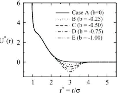
U*(r)
Case A (b=0) B (b = -0.25) C (b = -0.50) D (b = -0.75) E (b = -1.00)
FIG. 1. Interaction potential Eq.(1)with parametersa=5.0,r0/σ=0.7, c=1.0,r1/σ=3.0,andd=0.5 for all cases.bis shown in TableIfor each case.
How the addition of an attractive part in the potential affects the overall pressure–temperature phase diagram? In
order to answer this question in Secs. III–V, we obtain the
pressure–temperature phase diagram of the potentials
illus-trated in Fig.1where the attractive part is increased
system-atically without changing the core-softened part of the
poten-tial. This is done by fixing the parameters of Eq.(1):a =5.0,
r0/σ =0.7,c=1.0,r1/σ =3.0,d =0.5 and varying the
pa-rameterbas shown in TableIfor the five cases studied in this
work.
III. DETAILS OF SIMULATIONS
For the case in which b=0, the results shown in this
paper were adapted from Refs.35and49. For the other cases
(b=0) the details of the simulations go as follows.
The quantities of interest were obtained byNVT-constant
molecular dynamics using the LAMMPS package.58 The
system consists of N=1372 particles into a cubic box
with periodic boundary conditions in all directions. The
in-teraction potential between particles, Eq. (1), has a
cut-off of rc=4.5σ and the potential was shifted in order to
have U =0 at rc. The Nose–Hoover heat-bath with
cou-pling parameterQ =2 was used in order to keep fixed the
temperature.
All simulations were initialized in a liquid phase
previ-ously equilibrated over 5×10⁵ steps atT∗=0.6. The time
step used was 0.001 in reduced units and the runs were carried
out for a total of 3×10⁶steps, dumping instantaneous
con-figurations for every 2000 steps, giving then a total of 1500 independent configurations. The first 200 configurations were discarded for equilibration purposes, thus 1300 configurations were used for sampling averages. The highly number of inde-pendent configurations guarantees percentage uncertainty of
TABLE I. Parameterbin the potential Eq.(1)for each case studied in this work. The other parameters area=5.0,r0/σ=0.7,c=1.0,r1/σ=3.0, andd=0.5 for the five cases.
b
Case A 0
Case B −0.25
Case C −0.50
Case D −0.75
pressure and temperature of the isochores on PT diagram to be smaller than 1%. Thus, the uncertainties are smaller than the point size on PT diagram.
Preliminary simulations showed that depending on the chosen temperature and density, the system was in a fluid phase but became metastable with respect to the solid phase. In order to locate the phase boundary between the solid and the fluid phases, two sets of simulations were carried out, one beginning with the molecules in an ordered crystal structure and the other beginning with molecules in a random liquid state, obtained from previous equilibrated simulations. The stability of the system was checked by analyzing the depen-dence of pressure on density and also by visual analysis of the final structure, searching for cavitation.
The critical points were located as the locus where the isochores cross. The coexistence line between two different phases was estimated by the mean point between the spin-odals.
Temperature, pressure, density, and diffusion are mea-sured in dimensionless units,
T∗≡ kBT
ǫ ,
ρ∗≡ρσ3,
(2)
P∗≡ Pσ
3
ǫ ,
D∗≡ D(m/ǫ)
1/2
σ .
The pressure of the system is calculated by means of the the virial theorem,
P =ρkBT +
1
3V
i<j
f
ri j
·ri j
, (3)
whererij is the vector that connects particleiwith particlej,
f(r)=–∇U(r). The symbol...indicates ensemble average.
The mobility of particles is evaluated by the mean square displacement, given by
r(τ)2
=
[r(τ0+τ)−r(τ0)]2 . (4)
The diffusion coefficient is then obtained from Einstein’s relation, namely
D= lim
τ→∞
r(τ)2
6τ . (5)
For normal fluids, the diffusion at constant temperature grows with decreasing density. Actually in most cases it is expected that it would follow the Stokes–Einstein relation,
i.e.,D∝T.
The structure of the system was analyzed by using the translational order parameter, defined as8,25,59,60
t =
ξc
0
|g(ξ)−1|dξ, (6)
whereξ =rρ1/3 is the inter-particle distance divided by the
average separation between pairs of particlesρ−1/3. Hereg(ξ)
is the distribution function of pairs.ξcis the distance cutoff,
where we use half of the length of the simulation box,rc,
mul-tiplied byρ1/3
. Another alternative torcwould be the first or
the second peak in theg(r). Our choice is preferable, first,
be-cause it is the maximum distance allowed for the calculation
of g(r)61 giving us a better approach allowed fort. Second,
the peaks ofg(r) change place according to density and
tem-perature of the system. Thus additional work would be neces-sary to find such positions.
For the ideal gas, g=1 thust =0. As the system
be-comes more structured a long range order (g=1) appears
andt assumes large values. The translational order
parame-ter has its maximum value in the crystal phase. Therefore,t
gives a measurement of how close is the fluid close to the crystallization. For a fixed temperature normal fluids present
a monotonict(ρ) curve, increasing with density.
IV. RESULTS
In this section we show what is the effect of increasing the attractive part of the potential in the pressure–temperature phase diagram regarding: (a) the presence and location of dif-ferent phases and critical points; (b) the presence of a density anomalous region; (c) the presence of diffusion anomalous re-gion; (d) the presence of a structural anomalous region.
A. Phase diagram
Figures 2(a)–2(e) illustrates the pressure–temperature
phase diagram obtained through simulations for the cases
A–E using the potential shown in Fig.1. The gray lines are
the isochores. In all cases, at high temperatures the system ex-hibit a fluid phase and a gas phase. These two phases coexist at a first order line that ends at a critical point (open circle at figure) for B–E cases. At low temperatures and high pressures there are two liquid phases coexisting at a first order line (not shown) ending at a second critical point (filled point at figure) for C–E cases. These critical points are identified in the graph by the region where isochores cross. The location was also checked by the peak of the specific heat. The coexistence line between the gas and the liquid phases and between the low density liquid phase and the high density liquid phase (both illustrated as solid lines) were obtained as the mean point be-tween the respective spinodals.
At low pressures and temperatures, the region where no isochore is present the liquid phase is metastable or unstable against solid phases. Since polymorphism characterizes the CS potentials, a number of solid phases might be expected. Here we do not explore the stability of the different solids. Also, in the case E, the liquid–liquid phase transition appears at negative pressures. The negative pressure indicates that the system wants to contract but since the volume is fixed it is not possible.
The main effect of the increase of depth of the attractive
well at the location of the different phases in the P T phase
244506-4 Nunes da Silvaet al. J. Chem. Phys.133, 244506 (2010)
0 0.1 0.2 0.3 0.4 0.5 0.6 T*
0 0.5 1 1.5 2
P* (a)
0 0.2 0.4 0.6 0.8 T*
0 0.2 0.4 0.6 0.8 1
P*
(b)
0.2 0.4 0.6 0.8
T* 0
0.2 0.4 0.6
P*
(c)
0.3 0.4 0.5 0.6 0.7 0.8 T*
0 0.1 0.2
P*
(d)
1 1.2 1.4 1.6
T* 0
0.04 0.08
P* (e)
FIG. 2. Pressure-temperature phase diagram. The gray lines are the isochores. (a) Case A (b=0):ρ∗=0.04, 0.06, 0.07,. . ., and 0.20 from bottom to top. (b) Case B (b= −0.25):ρ∗=0.01, 0.015,. . ., and 0.165 from bottom to top. (c) Case C (b= −0.50): same as panel (b), (d) case D (b= −0.75): same as panel (b). (e) Case E (b= −1.00):ρ∗=0.02, 0.025,. . ., and 0.2 from bottom to top. The solid, bold line is theT M Dline, the dashed line marks the diffusion extrema and the dotted line bounds the region of structural anomaly. The filled and open circles are the liquid–liquid and liquid–gas critical points, respectively. The thin solid lines are the coexistence lines.
low density:
βP
ρ =1−2πρ
f(r)r2dr−8π
2ρ2
3
f(r)f(r′)f(|r−r′|) sinθr2r′2dr dr′dθ,
(7)
where f(r)=e−βU(r)−
1. This method allows to approach
toPρphase diagram from pair interaction potentialU(r). At
Pρphase diagram, critical points are located as
∂P
∂ρ =0,
(8) ∂2P
∂ρ2 =0.
The low density behavior obtained using the
clus-ter expansion is illustrated in Fig. 3. For T∗=0.60,
Fig. 3 shows the pressure–density phase diagram for b
=0.0,−0.25,−0.50,−0.75,−1.00 using the second and
the third virial. For b= −1.00 the unstable region of the
pressure–density phase diagram is large and the system at this temperature is deep in the liquid–gas coexistence region
of the pressure–temperature phase diagram. Forb= −0.75
the unstable region is present but is rather small. For b
=0.0,−0.25,and−0.50 no unstable region in the
pressure-density phase diagram is observed indicating that the
sys-tem is above the liquid–gas transition and that T =0.60 is
larger than the critical point temperature. The comparison
be-tween the cases with b=0.0,−0.25, and −0.50 suggests
that since the slope of the pressure–density phase diagram
increases as b increases, the liquid–gas critical temperature
decreases as b increases, Tc∗(b= −0.25)<Tc∗(b= −0.50) <T∗
c(b= −0.75)<T
∗
c(b= −1.00). Consequently, the
at-tractive part favors the liquid phase to exist for higher
temper-atures what is also observed in discontinuous potentials.62,63
Figure4obtained from the simulations summarizes the effect
of the attractive part in the location of the critical points in the pressure–temperature diagram.
At high densities where the liquid–liquid phase transi-tion is present, the cluster expansion with second and third
0.02 0.03 0.04 0.05
ρ∗
-0.4 -0.2 0 0.2
P*
b=0.0 b=-0.25 b=-0.50 b=-0.75 b=-1.00
0 0.4 0.8 1.2 T*
0 0.04 0.08 0.12
P*
C
E B
E
FIG. 4. Location of the critical points obtained usingNVTsimulations for the cases B–E considered in this work. The case A does not present any fluid-fluid critical point whereas the case B has a liquid–gas but no liquid-liquid critical point. The critical points were located by the crossing of the isochores. The symbols have the same meaning as in Figs.2(a)–2(e), i.e., filled and open circles mark the liquid–liquid and liquid–gas critical points, respectively. The arrows indicate the direction of increasing the attractive interaction.
virial is not appropriated. Simulations show that as b
de-creases the pressure needed to form the high density liquid phase, decreases. The attractive part favors the high density liquid phase over the low density liquid phase. The attraction leads in this case to a more compact liquid phase what is also
observed in discontinuous potentials.62,63
B. Density anomaly
In order to test for the presence of density anomaly, we proceed as follows. From the Maxwell relation,
∂V
∂T
P
= −
∂P
∂T
V
∂V
∂P
T
, (9)
the maximum in ρ(T) versus temperature at constant
pres-sure given by (∂ρ/∂T)P =0 is equivalent to the minimum of
the pressure versus temperature at constant density, namely
(∂P/∂T)ρ=0. While the former is suitable forNPT-constant
experiments/simulations the latter is more convenient for our
NVT-ensemble study, thus adopted in this work.
The temperatures of minimum pressure at constant den-sity or equivalently the temperatures of maximum denden-sity
at constant pressure, the TMD, obtained by NVT
simula-tions are illustrated in Figs.2(a)–2(d)as a bold line. As the
attractive well becomes deeper, the region in the pressure– temperature phase diagram occupied by the density anoma-lous region shrinks and moves to lower pressures and higher
temperatures until to the limiting case,b= −1.00, shown in
Fig.2(e), in which no density anomaly is present. This result
can be understood using the radial distribution function. The
T M D is related to the presence of large regions in the sys-tem in which particles are in two preferential distances repre-sented by the first scale and the second scale reprerepre-sented by the two first peaks in the radial distribution function in our potential.40,64–66
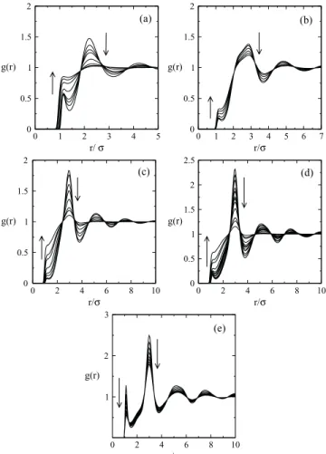
Figure5(e)illustrates the behavior expected for normal
liquids. As the temperature is increased the percentage of par-ticles in closest scales decreases. The decrease of parpar-ticles in the first scale leads to a decrease of density with the increase
of temperature. In Figs. 5(a)–5(d), as the temperature is
in-0 1 2 3 4 5
r/ σ
0 0.5 1 1.5 2
g(r)
(a)
0 1 2 3 4 5 6 7
r/σ
0 0.5 1 1.5 2
g(r)
(b)
0 2 4 6 8 10
r/σ
0 0.5 1 1.5 2
g(r)
(c)
0 2 4 6 8 10
r/σ
0 0.5 1 1.5 2 2.5
g(r)
(d)
0 2 4 6 8 10
r/σ
1 2 3
g(r)
(e)
FIG. 5. Radial distribution function obtained using NVT simula-tions vs distance for (a) case A (b=0.0) with ρ∗=0.14 and
T∗=0.25,0.35,0.45,0.55,1.0,2.0,3.0,and 4.0; (b) case B (b= −0.25) withρ∗=0.085 andT∗=0.32, 0.36, 0.44, 0.56, 0.68, and 0.80; (c) case C (b= −0.50) withρ∗=0.06 andT∗=0.44, 0.48, 0.60, 0.72, 1.0, 1.6, 2.0, and 3.5; (d) case D (b= −0.75) withρ∗=0.06 andT∗=0.40, 0.44, 0.48, 0.56, 0.60, 0.68, 0.72, 0.80, and 1.0; and (e) case E (b= −1.00) with ρ∗=0.07 and T∗= 0.45, 0.50, . . ., and 0.80. The arrows indicate the direction of increasing temperature.
creased the percentage of particles at the closest distance in-creases while the percentage of particles in the second scale decreases. The increase of particles in the first scale leads to an increase of density with temperature what characterizes the anomalous region. The density anomaly is, therefore, related to the increase of the probability of particles to be in the first scale when the temperature is increased while the percentage of particles in the second scale decreases. As the potential becomes highly attractive this “mobility” between scales dis-appears, i.e., the high density liquid becomes dominant and no anomalous region is observed.
C. Diffusion anomaly
The mobility was obtained from the slope of the mean
square displacement as shown in Eqs. (4) and(5). Figures
6(a)–6(e) show the behavior of the dimensionless
transla-tional diffusion coefficient, D∗, as the function of the
di-mensionless density,ρ∗, at constant temperature forb=0.0,
244506-6 Nunes da Silvaet al. J. Chem. Phys.133, 244506 (2010)
0.05 0.1 0.15 0.2
ρ∗
ρ∗ ρ∗
ρ∗
ρ∗
0.1 0.2 0.3
0.4 (a)
0.06 0.08 0.1 0.12
0 0.1 0.2 0.3 0.4 0.5
D* D*
D* D*
D*
(b)
0.04 0.06 0.08 0.1
0 0.2 0.4 0.6 0.8
(c)
0.04 0.06 0.08 0.1
0.15 0.2 0.25 0.3 0.35
0.4 (d)
0 0.04 0.08 0.12
0 0.5 1 1.5 2 2.5 3
(e)
FIG. 6. The diffusion coefficient against density for the (a) case A, with isotherms 0.2, 0.23, 0.262, 0.3, 0.35, 0.4, and 0.45 from bottom to top. (b) Case B with isotherms 0.16, 0.20,. . ., and 0.56, (c) case C, whose tem-peratures shown are 0.36, 0.40,. . ., and 0.68, (d) case D, with temperatures 0.48, 0.52,. . ., and 0.80, and (e) case E with isotherms 0.70, 0.75,. . ., 1.0, 1.10,. . ., and 1.70. The dashed lines mark the local maxima/minima in the D(ρ) curves. For the region enclosed by these lines particles move faster un-der compression. The dashed lines in this figure have the same meaning as those ones in Figs.2(a)–2(e). The diffusion coefficient was obtained from the slope of the mean square displacement versus time. The mean square dis-placement was obtained byNVTsimulations.
The solid lines are polynomial fits to the data obtained
through simulation [dots in Figs.4(a)–4(e)].
For normal liquids, the diffusion coefficient at constant temperature decreases with increase of the density. For the
cases A–D [shown in Figs. 4(a)–4(d)] D∗ anomalously
in-creases with the increase in the density in a certain range of
pressures and temperatures. From Figs.4(a)–4(d)show that
for very small and very high densities D∗ decreases with
increasing density as expected for a normal liquid. For
in-termediate values of density, ρDmax> ρ > ρDmin, D∗
in-creases with increasing density what leads to local maxima at
ρDmax and a local minima at ρDmin. These local extrema
in the diffusion versus density plots bound the region in-side which the diffusion behaves anomalously [dashed lines
in Figs.4(a)–4(d)]. This region is mapped into the pressure–
temperature diagram illustrated in Figs.2(a)–2(d)as dashed
lines in (a)–(d). As the attractive well becomes deeper, the diffusion anomalous region in the pressure–temperature phase
0.05 0.1 0.15 0.2 0.25 ρ∗
0.6 0.8 1 1.2
t
(a)
0.05 0.1 0.15 0.2 0.25 ρ∗
0.6 0.8 1 1.2 1.4
t
(b)
0.05 0.1 0.15 0.2
ρ∗
0.6 0.8 1 1.2
t
(c)
0.05 0.1 0.15 0.2 0.25 0.3
ρ∗
0.6 0.7 0.8 0.9 1 1.1 1.2
t
(d)
0.05 0.1 0.15 0.2 ρ∗
0.4 0.5 0.6 0.7 0.8 0.9 1 1.1
t
(e)
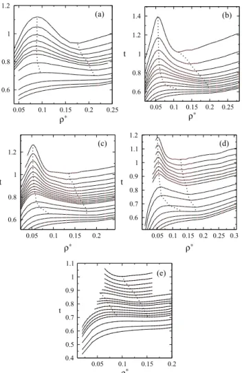
FIG. 7. Translational order parameter obtained byNVTsimulations against density for (a) case A, where each line correspond to an isotherm. The isotherms are: 0.25, 0.30,. . ., 0.55, 0.7, 1.0, 1.5, 2.0, and 2.5 from top to bottom. (b) Case B, with isotherms 0.20, 0.28,. . ., 0.68, 0.80, 1.0, 1.2, 1.6, 2.0, and 2.5 from top to bottom. (c) Case C whose temperatures are 0.36, 0.40,. . ., 0.80, 1.0, 1.2, 1.6, 2.0, 2.5, and 3.0 from top to bottom. (d) Case D withT∗=0.52, 0.56,. . . ,0.80, 1.0, 1.2, 1.6, 2.0, 2.5, 3.0, and 3.5 from top to bottom. Finally, (e) case E withT∗=0.70, 0.75,. . ., 1.0, 1.10,. . ., 1.70, 2.0, 2.5, and 3.0 from top to bottom. The dotted lines bound the region of structural anomalies, i.e., the region where the parametertdecreases upon increasing density.
diagram shrinks and it goes to lower pressures. In the case in
whichb= −1.00, shown in Fig.6(e), the diffusion constant
behaves as in a normal liquid. The diffusion anomalous re-gion lies, as one would expect, in the low density liquid phase where particles are less bound. As the attractive part of the potential becomes deeper, particles become more bound, fa-voring the high density liquid phase, and eliminating the pos-sibility of anomalous mobility.
D. Structural anomaly
Besides the density and the diffusion anomalies, a
struc-tural anomalous region might be present. Figures 7(a)–7(e)
show the translational order parameter defined by Eq.(6)as a
0 0.05 0.1 0.15 0.2 0.25 ρ∗
-1 -0.8 -0.6 -0.4 -0.2 0
s 2
0.04 0.08 0.12 ρ∗
-3 -2.5 -2 -1.5 -1 -0.5 0
s 2
0 0.05 0.1 0.15 0.2 0.25 ρ∗
-1.5 -1 -0.5 0
s 2
0 0.05 0.1 0.15 0.2 0.25 ρ∗
-1.2 -1 -0.8 -0.6 -0.4 -0.2 0
s 2
0 0.05 0.1 0.15 0.2 ρ∗
-0.6 -0.5 -0.4 -0.3 -0.2 -0.1 0
s 2
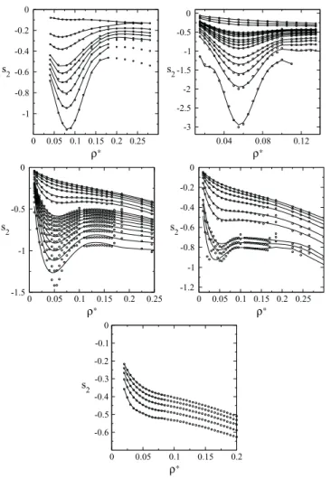
FIG. 8. Excess entropy vs density for:(a)b=0.00 andT∗=0.25,0.30,. . ., 0.7, 1.0, 3.0, and 5.0; (b)b= −0.25 andT∗=0.08, 0.10,. . ., 0.18, 0.24, 0.26, 0.28, 0.32, 0.36, 0.44, 0.48, 0.52, 0.54, 0.56, 0.64, 0.68, 0.72, 1.20, 1.60, and 2.50; (c)b= −0.50 andT∗=0.08, 0.10,. . ., 0.18, 0.24, 0.26, 0.28, 0.32, 0.36, 0.44, 0.48, 0.52, 0.54, 0.56, 0.64, 0.68, 0.72, 0.76, 0.80, 1.00, 1.20,1.60, 2.00, 2.50, and 3.00; (d)b= −0.75 andT∗=0.24, 0.26, 0.28, 0.32, 0.36, 0.40, 0.44,. . ., 0.80,1.00, 1.20,1.60, 2.00, 2.50, and 3.00; (e)b= −1.00 andT∗=1.10, 1.15, 1.20, 1.30,. . ., 1.70, 2.00, and 3.00.
The dots represent the simulation data and the solid lines are polynomial fit to the data.
The nonmonotonic behavior of these curves indicates
that there is a region in whicht decreases with density. This
means that the system becomes less structured for increas-ing density. Dotted lines determine the local maxima and
minima oft, bounding the structural anomalous region. This
region was mapped into the pressure–temperature phase
di-agram (dotted lines), as can be seen in Figs.2(a)–2(e). The
comparison between the behavior for differentbvalues
indi-cates that as the attractive well becomes deeper the structural anomalous region in the pressure–temperature phase diagram shrinks and moves to lower pressures and it is still present
even in the deepest case,b= −1.00. According to these
re-sults, we believe that forb<−1.00, i.e., cases in which the
attractive part is more intense than one showed in case E, the structural anomalous region will also vanish. This result again is consistent with the idea that a deeper attractive term favors the high density liquid phase.
0.05 0.1 0.15 0.2
ρ∗
0 1 2
Σ2
ρ
D
s2
0.04 0.06 0.08 0.1 0.12 0.14 ρ∗
-1 0 1 2
Σ2
ρ
D s2
0.04 0.06 0.08 0.1 0.12
ρ∗
-0.5 0 0.5 1 1.5
Σ2
ρ
D
s2
0.06 0.08 0.1 0.12
ρ∗
-1 0 1
Σ2
ρ
D s2
0 0.05 0.1 0.15
ρ∗
-0.3 -0.2 -0.1 0 0.1
Σ2
FIG. 9. Derivative of the excess entropy with respect to density vs den-sity for: (a)b=0.00 andT∗=0.25, 0.30,. . ., 0.5, 0.7, 1.0, 3.0, and 5.0; (b) b= −0.25 and T∗= 0.08, 0.10, . . ., 0.18, 0.20, 0.24, 0.28, 0.32, 0.36, 0.44, 0.48, 0.52, 0.54, 0.56, 0.64, 0.68, 0.72, 1.20, 1.60, and 2.50; (c)b= −0.50 andT∗=0.08, 0.10,. . ., 0.18, 0.24, 0.26, 0.28, 0.32, 0.36, 0.44, 0.48, 0.52, 0.54, 0.56, 0.64, 0.68, 0.72, 0.76, 0.80, 1.00, 1.20, 1.60, 2.00, 2.50, and 3.00; (d)b= −0.75 andT∗=0.24, 0.26, 0.28, 0.32, 0.36, 0.40, 0.44, 0.48, 0.52, 0.56, 0.60, 0.64, 0.68, 0.72, 0.76, 0.80, 1.00, 1.20, 1.60, 2.00, 2.50, and 3.00; (e)b= −1.00 andT∗=1.10, 1.15, 1.20, 1.30, 1.40, 1.50, 1.60, 1.70, 2.00, and 3.00.
Complementary to the structural anomalous region
ob-tained by analyzing the parameter t, we can gain some
un-derstanding about the presence or absence of these anomalies and the shape of the potential by analyzing the density
depen-dence of the excess entropy.67 The excess entropy is defined
as the difference between the entropy of the real fluid and that of an ideal gas at the same temperature and density. Erring-tonet al.have shown that the density anomaly is given by the
conditionex=(∂sex/∂lnρ)T >1.67 They have also shown
that the two body contribution ofsex,
sex≈s2= −2πρ
[g(r) lng(r)−g(r)+1]r2dr , (10)
gives a good approximation of sex. The radial distribution
function, g(r), is proportional to the probability to find a
particle at a distancer to another particle placed at the
ori-gin. Erringtonet al.67 have also suggested that the diffusion
anomaly can be predicted by using the empirical Rosenfeld’s
parametrization.68They found the condition
244506-8 Nunes da Silvaet al. J. Chem. Phys.133, 244506 (2010)
0 0.3 0.6 0
0.2 0.4 0.6 0.8 1
P*
0.3 0.6
T* 0 0.2 0.4 0.6 0.8 1
1 2 3 0
0.5 1 1.5 2 2.5
(a) (c)
A
B
D C
A
B C D
A
B
C D
E (b)
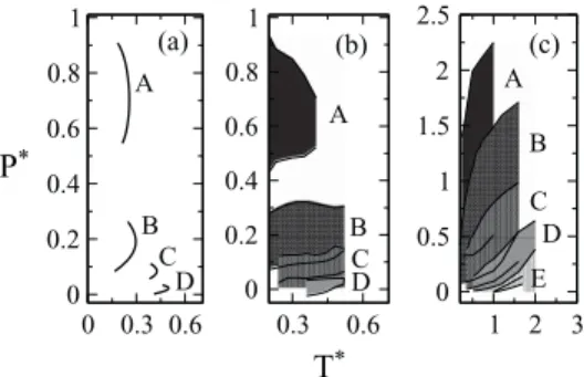
FIG. 10. (a)TMDline for the cases considered in this paper. Note that there is no density anomaly in the case E [see Figs.2(a)–2(e)]. (b) The diffusion anomaly region for the cases A–D. No diffusion anomaly was found for the case E [see Figs.6(a)–6(e)]. The shadowed regions correspond to the region between the dashed lines in Figs.2(a)–2(e). In (c) is shown the structural anomalous region for cases A–E. Here, the shadowed region corresponds to the region between the dotted lines in Figs.2(a)–2(e). All these results were obtained byNVTsimulations.
diffusion anomalous behavior. They also claim that2>0 is
a good estimate for determining the region where structural
anomaly occurs.67
Here we test these assumptions in our potential for the different depth of the attractive term.
Figures 8(a)–8(e) illustrate the excess entropy
ver-sus density for the cases b=0,−0.25,−0.50,−0.75
and b=1.0 for various temperatures. For the case b
=0,−0.25,−0.50,−0.75,the excess entropy as a function
of density has a range of temperatures and densities where the excess entropy has positive slope.
Figures 9(a)–9(e) illustrate the derivative of the excess
entropy with respect to the density versus density for the
cases b=0,−0.25,−0.50,−0.75 and b=1.0 for various
temperatures. For the casesb=0,−0.25,−0.50,−0.75 the
derivative of the excess entropy as a function of density
has a range of temperatures and densities where 2>1,
2 >0.42, 2>0 what indicates the presence of density,
diffusion, and structural anomalous regions. This is not the
case forb=1.0.
Figure 10 gives an overview of the density, diffusion,
and structural anomaly locations in the pressure–temperature phase diagram.
V. CONCLUSIONS
In this paper, we have explored the effect of the addition of an attractive part in a two length scale potential. Partic-ularly we analyze if the depth of the attractive part changes the position (and the presence or not) of the two liquid–gas and liquid–liquid critical points and of the density, diffusion, and structural anomalous regions in the pressure–temperature phase diagram.
Our results show that the depth of attractive part of pair interaction potential is directly related with the low density liquid. Analyzing the evolution of liquid–gas critical point at
P T phase diagram, we noted that it moves out to higher
tem-peratures as the attractive part of pair potential increase. The increase of the deep brings stability to the low density liquid phase. Thus, more energy is necessary to push out the system
from this state. When this energy is given through an increase of temperature, the system goes to the gas phase.
The main effect of the pressure is to keep particles close to the equilibrium point of the repulsive part. This makes it possible for the particles to move from the attractive part to the repulsive part of the potential. As the well becomes deeper, particles are trapped in the minimum of the attractive part. Hence a high pressure is not necessary to keep particles closer to the repulsive shoulder.
For sufficiently intense attraction between particles, both the liquid–liquid and the liquid–gas critical points are present. These two critical points are observed even for a very at-tractive potential. For a small atat-tractive interaction, only the liquid–gas critical point was found what indicates that for the coexistence of two liquid phases the attractive well have to be deeper than a certain threshold.
Since the attraction favors the liquid phase (particularly
the high density liquid phase), as theb decreases the liquid–
gas critical point moves to higher temperatures (shown in
Fig.4) and the liquid–liquid critical point to lower pressures.
The density, diffusion, and structural anomalous regions
are present even in the absence of attraction. As b
de-creases, the high density liquid structure is favored and so the anomalous regions in the pressure–temperature phase
di-agram (shown in Fig.10) shrinks, moves to lower pressures,
and disappears for very attractive potentials. The analysis of the excess entropy with density supports these results.
In order to resume, the density and the diffusion anoma-lies are present in systems which interact through two length scale potentials if the particle move from one scale to the other. If the attractive scale is too deep, the flux of particles between the scales decreases and no anomalies are observed.
VI. ACKNOWLEDGMENTS
We thank for financial support from the Brazilian science agencies CNPq, CAPES and FAPEMIG. This work is also partially supported by the CNPq through the INCT-FCx.
1Periodic table of the elements, http://periodic.lanl.gov/default.htm, 2007. 2R. Waler,Essays of Natural Experiments(Johnson Reprint, New York,
1964).
3F. X. Prielmeier, E. W. Lang, R. J. Speedy, and H.-D. Lüdemann,Phys.
Rev. Lett.59, 1128 (1987).
4L. Haar, J. S. Gallangher, and G. Kell,NBS/NRC Steam Tables. Thermo-dynamic and Transport Properties and Computer Programs for Vapor and Liquid States of Water in SI Units, 1st ed. (Hemisphere, Washington, DC, 1984).
5C. A. Angell, E. D. Finch, and P. Bach,J. Chem. Phys.65, 3063 (1976). 6P. A. Netz, F. W. Starr, H. E. Stanley, and M. C. Barbosa,J. Chem. Phys.
115, 344 (2001).
7P. A. Netz, F. W. Starr, M. C. Barbosa, and H. E. Stanley,Journal of
Molec-ular Liquids101, 159 (2002).
8J. R. Errington and P. G. Debenedetti,Nature (London)409, 318 (2001). 9J. Mittal, J. R. Errington, and T. M. Truskett,J. Phys. Chem. B110, 18147
(2006).
10A. Mudi, C. Chakravarty, and R. Ramaswamy,J. Chem. Phys.122, 104507 (2005).
11H. J. C. Berendsen, J. R. Grigera, and T. P. Straatsma,J. Phys. Chem.91, 6269 (1987).
12O. Mishima,J. Chem. Phys.100, 5910 (1994).
13O. Mishima and H. E. Stanley,Nature (London)396, 329 (1998). 14P. H. Poole, F. Sciortino, U. Essmann, and H. E. Stanley,Nature (London)
15P. A. Netz, F. W. Starr, M. C. Barbosa, and H. E. Stanley,Physica A314, 470 (2002).
16O. Mishima and H. E. Stanley,Nature392, 164 (1998). 17H. Thurn and J. Ruska,J. Non-Cryst. Solids22, 331 (1976). 18G. E. Sauer and L. B. Borst,Science158, 1567 (1967).
19S. J. Kennedy and J. C. Wheeler,J. Chem. Phys.78, 1523 (1983). 20T. Tsuchiya,J. Phys. Soc. Jpn.60, 227 (1991).
21P. T. Cummings and G. Stell,Mol. Phys.43, 1267 (1981). 22M. Togaya,Phys. Rev. Lett.79, 2474 (1997).
23C. A. Angell, R. D. Bressel, M. Hemmatti, E. J. Sare, and J. C. Tucker,
Phys. Chem. Chem. Phys.2, 1559 (2000).
24R. Sharma, S. N. Chakraborty, and C. Chakravarty,J. Chem. Phys.125, 204501 (2006).
25M. S. Shell, P. G. Debenedetti, and A. Z. Panagiotopoulos,Phys. Rev. E 66, 011202 (2002).
26S. Sastry and C. A. Angell,Nature Mater.2, 739 (2003).
27S. H. Chen, F. Mallamace, C. Y. Mou, M. Broccio, C. Corsaro, A. Faraone, and L. Liu,Proceedings of the National Acad. Sci. U.S.A.103, 12974 (2006).
28T. Morishita,Phys. Rev. E72, 021201 (2005).
29S. V. Buldyrev and H. E. Stanley,Physica A330, 124 (2003).
30A. Skibinsky, S. V. Buldyrev, G. Franzese, G. Malescio, and H. E. Stanley,
Phys. Rev. E69, 061206 (2005).
31V. B. Henriques, N. Guissoni, M. A. Barbosa, M. Thielo, and M. C. Bar-bosa,Mol. Phys.103, 3001 (2005).
32P. C. Hemmer and G. Stell,Phys. Rev. Lett.24, 1284 (1970). 33E. A. Jagla,Phys. Rev. E58, 1478 (1998).
34N. B. Wilding and J. E. Magee,Phys. Rev. E66, 031509 (2002). 35A. B. de Oliveira, P. A. Netz, T. Colla, and M. C. Barbosa,J. Chem. Phys.
124, 084505 (2006).
36N. G. Almarza, J. A. Capitan, J. A. Cuesta, and E. Lomba,J. Chem. Phys. 131, 124506 (2009).
37D. Y. Fomin, N. V. Gribova, V. N. Ryzhov, S. M. Stishov, and D. Frenkel,
J. Chem. Phys.129, 064512 (2008). 38G. Franzese,J. Mol. Liq.136, 267 (2007).
39A. B. de Oliveira, G. Franzese, P. A. Netz, and M. C. Barbosa,J. Chem.
Phys.128, 064901 (2008).
40A. B. de Oliveira, P. A. Netz, and M. C. Barbosa,Europhys. Lett.85, 36001 (2009).
41S. Zhou,Phys. Rev. E74, 031119 (2006). 42S. Zhou,Phys. Rev. E77, 041110 (2008). 43S. Zhou,J. Chem. Phys.130, 054103 (2009). 44S. A. Egorov,J. Chem. Phys.128, 174503 (2008).
45N. V. Gribova, Y. D. Fomin, D. Frenkel, and V. N. Ryzhov,Phys. Rev. E 79, 051202 (2009).
46E. G. Noya, C. Vega, J. P. K. Doye, and A. A. Louis,J. Chem. Phys.127, 054501 (2007).
47S. V. Buldyrev, G. Malescio, C. A. Angell, N. Giovambattista, S. Prestipino, F. Saija, H. E. Stanley, and L. Xu,J. Phys.: Condens. Matter
21, 504106 (2009).
48E. Lomba, N. G. Almarza, C. Martin, and C. McBride,J. Chem. Phys.126, 244510 (2007).
49A. B. de Oliveira, P. A. Netz, T. Colla, and M. C. Barbosa,J. Chem. Phys. 125, 124503 (2006).
50A. B. de Oliveira, M. C. Barbosa, and P. A. Netz,Physica A386, 744 (2007).
51A. B. de Oliveira, P. A. Netz, and M. C. Barbosa,European Physical Jouranl
B64, 481 (2008).
52A. B. de Oliveira, E. Salcedo, C. Chakravarty, and M. C. Barbosa,J. Chem.
Phys.132, 234509 (2010).
53A. B. de Oliveira, E. Salcedo, C. Chakravarty, and M. C. Barbosa,J. Chem.
Phys.132, 234509 (2010).
54W. P. Krekelberg, J. Mittal, V. Ganesan, and T. M. Truskett,Phys. Rev. E 77, 041201 (2008).
55Z. Yan, S. V. Buldyrev, P. Kumar, N. Giovambattista, P. G. Debenedetti, and H. E. Stanley,Phys. Rev. E76, 051201 (2007).
56C. H. Cho, S. Singh, and G. W. Robinson, Faraday Discuss. 103, 19 (1996).
57P. A. Netz, J. F. Raymundi, A. S. Camera, and M. C. Barbosa,Physica A 342, 48 (2004).
58S. J. Plimpton,J. Comp. Phys.117, 1 (1995).
59T. M. Truskett, S. Torquato, and P. G. Debenedetti,Phys. Rev. E62, 993 (2000).
60J. E. Errington, P. G. Debenedetti, and S. Torquato,J. Chem. Phys.118, 2256 (2003).
61D. Frenkel and B. Smit, Understanding Molecular Simulation, 1st ed. (Academic, San Diego, 1996).
62G. Malescio, G. Franzese, G. Pellicane, A. Skibinsky, S. V. Buldyrev, and H. E. Stanley,J. Phys.: Condens. Matter14, 2193 (2002).
63G. Malescio, G. Franzese, A. Skibinsky, S. V. Buldyrev, and H. E. Stanley,
Phys. Rev. E71, 061504 (2005).
64H. E. Stanley, S. V. Buldyrev, M. Canpolat, M. Meyer, O. Mishima, M. R. Sadr-Lahijany, A. Scala, and F. W. Starr,Physica A257, 213 (1998). 65H. E. Stanley,Pramana: Journal of Physica53, 53 (1999).
66H. E. Stanley, S. V. Buldyrev, M. Canpolat, O. Mishima, A. Sadr-Lahijany, M. R. Scala, and F. W. Starr,Phys. Chem. Chem. Phys.2, 1551 (2000).
67J. R. Errington, T. M. Truskett, and J. Mittal,J. Chem. Phys.125, 244502 (2006).