Metropolitan Area
Cleomar Gomesda silva Fábio auGusto reis Gomes
Resumo
Este artigo usa modelos ARFIMA e testes de raiz unitária com quebra estrutural para examinar o grau de persistência do desemprego de diferentes estratos da força de trabalho na Região Metropolitana de São Paulo. Para tanto, a taxa agregada desta região é examinada, como também sua desagregação por gênero, idade, raça e posição dentro da família. O período de análise vai de janeiro de 1985 a novembro 2008 e, apesar do uso de diferentes métodos de estimação, a hipótese de raiz unitária não é rejeitada em geral. As duas exceções são as séries relacionadas aos trabalhadores entre 15 e 17 anos e acima dos 40 anos. Mas, mesmo nestes dois casos, o parâmetro "d" fica acima de 0,5. Isso indica que não há estacionariedade e também não há reversão a uma média de longo prazo para a maioria das séries analisadas. Portanto, as políticas econômicas de combate à inflação das últimas duas décadas, assim como mudanças em variáveis reais, têm gerado efeitos duradouros sobre a taxa de desemprego em São Paulo.
PalavRas-Chave
desemprego, persistência, memória longa, raiz unitária
abstRaCt
This article makes use of ARFIMA models and unit root tests with structural breaks to examine the un-employment persistence of different labor forces in the Greater Metropolitan Area of São Paulo. To this purpose, not only is the region’s open unemployment rate analyzed but it is also disaggregated by gender, age, color and position within the household. The period ranges from January 1985 to November 2008 and, despite using a range of estimation methods, the presence of a unit root cannot be rejected in general. The exceptions are the series related to Age 15-17 and over 40. But even in these cases the parameter "d" lies above 0.5. This is an indication that the unemployment rates in São Paulo can be defined as non stationary and the majority of the series are not mean-reverting. Therefore, the disinflation policies imple-mented by the Brazilian policymakers in the last two decades, as well as changes in real variables, have had long-lasting effects on the unemployment rates in São Paulo.
KeywoRds
unemployment, persistence, long memory, unit root.
Jel ClassifiCation
C32, E24
Fundação Getulio Vargas de São Paulo. Endereço para contato: Rua Itapeva 474, 11º andar, São Paulo – SP. E-mail:
Insper Instituto de Ensino e Pesquisa. Endereço para contato: Rua Quatá 300, São Paulo – SP. E-mail: FabioARG@
insper.org.br
1 IntRoDuctIon
The Greater São Paulo Metropolitan Area is one of the five most populous places in the world. According to the 2006 estimate released by IBGE, the Brazilian Bureau of Geography and Statistics, the region has a population of around 19 million peo-ple in its 55 municipalities and the city of São Paulo itself has a population of over 11 million. Therefore, the Greater São Paulo Metropolitan Area accounts for about 10% of the total Brazilian population. Such magnitude has made unemployment an important issue, especially in the last two decades. And this is due to many fac-tors, such as a series of failed economic stabilization plans in the 1980s and in the beginning of the 1990s.
The implementation of the Real Plan, in 1994, can be considered to be the tur-ning point in the Brazilian economy, once it was the first stabilization package that really managed to bring down inflation in the country. Nonetheless, Brazilian policymakers opted to keep an appreciated fixed exchange rate, which culminated in serious consequences to the trade balance account, level of international reserves and unemployment rates as well. All of these factors together, and a deep interna-tional crisis, forced the country to adopt a flexible exchange rate in 1999. Shortly after the exchange rate depreciation, the Brazilian central bank adopted an inflation targeting regime so as to build credibility on its intention to fight inflation and put the country back on the track.
Theoretically, NAIRU and Hysteresis are the two main hypotheses related to the ex-planation of unemployment and its persistence. Friedman (1968) and Phelps (1968) proposed the Natural Rate Hypothesis, arguing that real variables determined their own behavior and, consequently, they could not be influenced permanently by nomi-nal variables, such as inflation. As a result, unemployment would converge to its natural rate in the long run, i.e., it should be a non-integrated process, I(0), with transitory shocks. On the other hand, Blanchard and Summers (1986) showed that the insider’s bargaining power in wage-setting implied that aggregate employment is a random walk process with a drift. In this case, the unemployment rate would be an integrated process, I(1), and any shock to the series would shift unemployment equilibrium permanently from one level to another. This persistence is what defines the so-called Hysteresis phenomenon.1 In other words, perturbations affecting
un-employment can be either transitory (NAIRU) or permanent (Hysteresis) and the
degree of persistence they generate is a key determinant of the costs of disinflation policies.
As far as econometrics is concerned, the two theories stated in the previous paragra-ph can be evaluated by means of unit root tests, in which the order of integration
d of the unemployment rate is tested. There is even the possibility to use unit root tests which take into account structural breaks. This was done in several articles such as: Neudorfer et al. (1990), Mitchell (1993), Jaeger and Parkinson (1994), Song and Wu (1998), Arestis and Mariscal (1999), Camarero and Tamarit (2004), Clement et al. (2005). For the Brazilian, there are, among others, Gomes and Gomes da Silva (2008; 2009).
However, this methodology imposes that d assumes an integer value, i.e., unem-ployment is either I(0) or I(1), and discards the possibility of a non-integer parame-ter. Auto-Regressive-Fractionally-Integrated-Moving-Average (ARFIMA) models account for this matter, allowing for a fractional difference parameter d. This me-thodology helps to overcome the well-known problem of low power of traditio-nal unit roots and also helps to jointly model short-run and long-run dynamics of unemployment.
However, these researches do not take into consideration that possibility that the persistence detected by the ARFIMA model can be caused by structural breaks in the series. Theoretically, the importance of analyzing such possibility has been done by Diebold and Inoue (2001), who wrote that the long-memory literature has not paid enough attention to the possibility of confusing structural breaks and long memory processes. Granger and Hyung (2004) also approached the same problem, showing that omitting occasional breaks leads to an overestimated d. For instance, Baum, Barkoulasb and Caglayanc (1999) analyzed the real exchange rate of several countries in the post-Bretton Woods era, concluding that the unit-root hypothesis is robust against both fractional alternatives and structural breaks. Asikainen (2003) did something for the Finnish and Swedish party popularity series. According to the author’s findings, three series tested had structural breaks and, in two cases, the control of the breaks changed the unit root assumption to a fractional unit root.
This study attempts to fill this research gap for the Brazilian case.2 To this purpose, this article makes use of unit root tests with structural breaks as well as ARFIMA models to examine the unemployment persistence of different labor forces in the Greater Metropolitan Area of São Paulo.3 The period analyzed ranges from January
1985 to November 2008 and not only is the region’s open unemployment rate analyzed but it is also disaggregated by gender, age, color and position within the household. Despite using a range of estimation methods, the presence of unit root cannot be rejected in general. The exceptions are the series related to Age 15-17 and over 40. But even in these cases the parameter d lies above 0.5. This is an indication that the unemployment rates in São Paulo can be defined as non stationary and the majority of the series are not mean-reverting. Hence, all disinflation policies perfor-med by the Brazilian policymakers in the last two decades, and also technological changes, have impacted São Paulo’s labor force systematically, spreading through all kinds of workers.
The remainder of the paper is organized as follows. Section 2 presents the econo-metric methodology. Section 3 presents the data. Section 4 summarizes the results and section 5 concludes the article.
2 For the Brazilian case, we are unaware of studies comparing hysteresis and NAIRU. But there are pa-pers related to NAIRU only. For example, Portugal and Madalozzo (2000) and Lima (2000) did not confirm the NAIRU hypothesis, which might be an indication that the hysteresis theory may be the case.
2 EconoMEtRIc MEtHoDoloGY
2.1. aRFIMa Models
Define Xi t, =1, if individual i is unemployed in period t and Xi t, =0, otherwise.
Thus, if
i
=
1
,...,
N
, aggregate unemployment can be defined as an aggregation of apanel data information of the kind:
, 1
/
Nt i t
i
u
X
N
=
=
∑
(1)As usual, suppose that Xi t, follows a Markov Process with transition probabilities
given by:
, ,
, ,
t t
e e u e
t t
e u u u
p
p
p
p
(2)where , t s k
p is the probability of changing from regime s to regime k in period t, and
e refers to being employed while u refers to being unemployed.4 The probabilities depend on t due to aggregate shocks, such as those coming from monetary policy. Finally, if for each period the Markov Process is ergodic, then:
( )
, ,
1
/
Nt i t i t
i
u
X
N
E X
=
=
∑
→
(3)where
( )
, , ,t t
i t e u u u
E X
=
p
+
p
is the probability of becoming unemployed plus theprobability of continuing unemployed.
Applying the ARFIMA methodology to the unemployment rate is equivalent to modeling the probability above, with special interest in measuring its degree of persistence. Therefore, suppose that
{
u t
t,
=
1, 2,...,
T
}
is the observed unemploymenttime series that follows the model:
(
1
−
L
)
du
t=
e
t (4)where et is a covariance stationary process and d can be any real number. If this the case, the operator (1 - L)-d can be represented by the filter:
(
)
0
1
d j jj
L
L
∞ −
=
−
=
∑
λ
(5)where λ0 ≡ 1,
λ =
j(
1 / !
j
)(
d
+ −
j
1
)(
d
+ −
j
2
)(
d
+ −
j
3
) (
d
+
1
)( )
d
and, as aresult,
(
1
)
0 1 1 2 2d
t t t t t
u
= −
L
−e
= λ
e
+ λ
e
−+ λ
e
−+
(6)Notice that the parameter d plays a central role in explaining the impact of past shocks on
u
t. In fact, ife
t is a white noise, equation (6) gives the impulse responsefunctions of ut. Whilst the impulse-response coefficients for a stationary ARMA process decay geometrically, the ARFIMA process has a slower (hyperbolic) decay. Because of this feature, fractionally integrated processes can be useful in modeling time series with long memory.
In the ARFIMA framework5, the higher the order of integration of the series, the
higher its persistence will be. In fact, if 0 ≤ d ≤ 0.5, the series is stationary and
mean-reverting. If 0.5 < d < 1, the series is non-stationary but still mean-reverting (the effects of shocks are long-lasting). Finally, when d ≥ 1, the series is
non-stationary and non-mean-reverting (GIL-ALANA, 2001a).
In order to estimate the parameter d the Nonlinear Least Squares Method (NLS) - sometimes referred to as the Approximate Maximum Likelihood Method - is used.6 The NLS estimator is based on the maximization of the following likelihood function:
(
)
1
1
1
, ,
log
2
N
N t
i
d
e
T
=
Φ Θ = −
∑
(7)5 The reader may refer to Granger and Joyeux (1980) and Hosking (1981) for a complete understanding of the fractionally integrated models.
where the residuals et are obtained by applying the ARFIMA(p, d, q) to ut and the
vectors
Φ
and Θ represent the p autoregressive and the q moving-average param-eters, respectively.72.2. structural Breaks
Besides examining whether the disaggregated unemployment rate series have long memory properties, we have to check whether these series have structural breaks. This is important once, as mentioned, one may conclude that a series has a long memory process when it is influenced by structural breaks.
In order to examine the order of integration of the unemployment series, we follow the same procedure applied in Gomes and Gomes da Silva (2008). We first apply unit root tests, such as ADF and KPSS. However, since Perron (1989), it is well known that ADF tests can fail to reject a false unit root due to misspecification of the deterministic trend. In fact, Perron (1989, 1997) and Zivot and Andrews (1992) extend the ADF test considering an exogenous and an endogenous break to avoid this problem. But these types of tests also have some drawbacks once they derive their critical values assuming no break(s) under the null hypothesis, which lead to a spurious rejection of the null hypothesis in the presence of a unit root with breaks (LEE; STRAZICICH, 2001).
Therefore, we decided to make use of an endogenous two-break LM unit root test proposed in Lee and Strazicich (2003). In contrast to the ADF-type tests, the pro-perties of these LM tests are unaffected by breaks under the null. According to the LM (score) principle, a unit root test statistic can be obtained from the following regression:
1 1 '
k
t t t i t i t
i
u g Z S− S−
=
∆ = ∆ + ϕ +
∑
γ ∆ + ε (8)where: i)
S
~
t is a de-trended series such that St = − ψ − δ =ut x Zt,t 2,...,T ; ii) δ isa vector of coefficients in the regression of Δut on
∆
Z
tand ψ = − δx u1 Z1, wheret
Z
is defined below; iii)u1 andZ
1 are the first observations of ut andZ
t,respec-tively. iv)
∆
S
t i−(
where i
=
1,...,
k
)
terms are included as necessary to correct for serial correlation; v)Z
t is a vector of exogenous variables defined by the datanerating process. Considering two changes in level and trend,
Z
t is described by1 2 1 2
1, ,t D Dt, t,DT DT∗t, ∗t ′
, where Djt =1for t≥TBj+1, j = 1,2, and zero otherwise, jt
DT∗=t for t≥TBj+1, j = 1, 2, and zero otherwise, and TBjstands for the time
pe-riod of the breaks. Note that the test regression (8) involves ∆Ztinstead of
Z
t sothat
∆
Z
t becomes 1,B B1t, 2t,D D1t, 2t′
, where Bjt =∆Djt and Djt DTjt,j 1, 2 ∗
= ∆ = .
The unit root null hypothesis is described in equation (8) by ϕ =0and the test statistics is defined as ρ = ⋅φ T . For the null hypothesis
(
φ =
0
)
, τ= t-statistic. To endogenously determine the location of the two breaks(
λ =j TBj / ,T j=1, 2)
we use the LMτ = Infλτ λ( ). As in Lee and Strazicich (2003), we use critical values that correspond to the location of the breaks, (λ =j TBj T j, =1, 2)3 Data
The data used in the analysis are the seasonally adjusted monthly unemployment ra-tes of different labor forces in the Greater Metropolitan Area of São Paulo. The time series are the following: i) male; ii) female; iii) white; iv) non-white; v) head of the household; vi) other members of the household; vii) workers aged 15 to 17, 18 to 24, 25 to 39 and over 40; viii) aggregate open unemployment rate. The data were obtai-ned from SEADE (Fundação Sistema Estadual de Análise de Dados) and the sample period ranges from 1985:01 to 2008:11, giving a total of 287 observations.
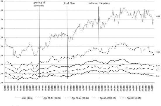
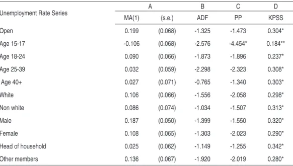
Figure 1 shows the evolution of unemployment in the São Paulo Metropolitan Area. The rates of unemployment of other members of household, female and nonwhite workers8 are the highest. On the other hand, male, white and head of household workers have lower rates. Figure 2 shows the rates of unemployment of different age groups of workers. It is clear that youngsters have higher unemployment rates than older workers9. Hence, what the two figures suggest is that the Real Plan did not have a negative effect on employment until the end of 1995. From then on, there was an increase in unemployment, which lasted until the end of 1998. From the beginning of 1999, the period of adoption of a flexible exchange rate followed by the implementation of the inflation targeting regime, unemployment rates became instable again and, after 2003, they started to show some decrease.
8 As a matter of fact, nonwhite workers have usually unemployment rates higher than whites, even when qualification differences are taken into consideration.
FIGuRE 1 – sEasonallY aDjustED unEMPloYMEnt sERIEs (1985:01 to 2008:11) 3,37 12.95 6,69 11.51 8,51 9,80 0,00 2,00 4,00 6,00 8,00 10,00 12,00 14,00 16,00 18,00 20,00 19 85 M0 1 19 85 M1 0 19 86 M0 7 19 87 M0 4 19 88 M0 1 19 88 M1 0 19 89 M0 7 19 90 M0 4 19 91 M0 1 19 91 M1 0 19 92 M0 7 19 93 M0 4 19 94 M0 1 19 94 M1 0 19 95 M0 7 19 96 M0 4 19 97 M0 1 19 97 M1 0 19 98 M0 7 19 99 M0 4 20 00 M0 1 20 00 M1 0 20 01 M0 7 20 02 M0 4 20 03 M0 1 20 03 M1 0 20 04 M0 7 20 05 M0 4 20 06 M0 1 20 06 M1 0 20 07 M0 7 20 08 M0 4
head (3.37) other members (12.95) male (6.69)
female (11.51) White (8.51) Non white (9.80)
opening of
economy Real Plan TargetingInflation
Source: Seade.
FIGuRE 2 - sEasonallY aDjustED unEMPloYMEnt sERIEs (1985:01 to 2008:11) 8,85 35,29 15,92 7,11 3,61 0,00 5,00 10,00 15,00 20,00 25,00 30,00 35,00 40,00 45,00 19 85 M 01 19 85 M 07 19 86 M 01 19 86 M 07 19 87 M 01 19 87 M 07 19 88 M 01 19 88 M 07 19 89 M 01 19 89 M 07 19 90 M 01 19 90 M 07 19 91 M 01 19 91 M 07 19 92 M 01 19 92 M 07 19 93 M 01 19 93 M 07 19 94 M 01 19 94 M 07 19 95 M 01 19 95 M 07 19 96 M 01 19 96 M 07 19 97 M 01 19 97 M 07 19 98 M 01 19 98 M 07 19 99 M 01 19 99 M 07 20 00 M 01 20 00 M 07 20 01 M 01 20 01 M 07 20 02 M 01 20 02 M 07 20 03 M 01 20 03 M 07 20 04 M 01 20 04 M 07 20 05 M 01 20 05 M 07 20 06 M 01 20 06 M 07 20 07 M 01 20 07 M 07 20 08 M 01 20 08 M 07
open (8.85) Age 15-17 (35.29) Age 18-24 (15.92) Age 25-39 (7.11) Age 40+ (3.61)
opening of
economy Real Plan Inflation Targeting
Table 1 helps us to analyze unemployment behavior more carefully. It reports the unemployment mean and growth rates considering full and sub samples of the se-ries. Looking at the full sample, unemployment amongst youngsters aged between 15 and 17 has the highest mean, followed by workers aged between 18 and 24 and other members of household. On the other hand, the head of household’s unem-ployment rate is the lowest, which is expected once these workers have a higher op-portunity cost of waiting for a better job offer when they do lose their jobs. As for workers over 40 years of age, their rate of unemployment is also low because they are very experienced, which increases their marginal product. White workers have a lower rate of unemployment than non-whites, which is a common finding even when human capital accumulation is taken into account. Finally, the unemployment rate of males is much lower than of females.
ta BlE 1 – sE ason a llY a Dj ustED u nE M PloYM Ent sER I Es: DEscRIPtIvE statIstIcs
Unemployment Rate Series
Mean Growth Rate
Whole Sample
Sub Sample 1
Sub Sample 2
Sub
Sample 3 Sub Sample 1 to Sub Sample 2
Sub Sample 2 to Sub Sample 3
Sub Sample 1 to Sub Sample 3 1985:01 to
2008:11
1985:01 to 1994:06
1994:07 to 1998:12
1999:01 to 2008:11
Open 9.47 7.48 10.03 11.13 34.11% 10.97% 48.82%
Age 15-17 28.53 20.24 28.93 36.29 42.91% 25.44% 79.26%
Age 18-24 14.87 10.71 15.17 18.73 41.66% 23.51% 74.96%
Age 25-39 6.77 5.00 7.19 8.27 43.97% 14.96% 65.51%
Age 40+ 4.45 3.03 4.78 5.67 57.92% 18.50% 87.13%
White 8.66 6.93 9.13 10.10 31.60% 10.71% 45.70%
Non white 10.97 8.63 11.73 12.86 35.94% 9.59% 48.97%
Male 7.56 6.15 8.17 8.65 32.81% 5.84% 40.57%
Female 11.99 9.51 12.58 14.10 32.27% 12.14% 48.32%
Head of
household 4.20 3.15 4.68 4.99 48.66% 6.51% 58.34%
Other members 13.41 10.75 14.04 15.67 30.55% 11.64% 45.75%
Source: Seade.
4 REsults
First of all, it is advisable to plot the sample autocorrelations and investigate them carefully. They are reported, in levels and in first differences, on Table 2. In levels, the values begin at 0.98 or 0.99 and then decay very slowly. In fact, at lag 18 all of them are still above 0.70, which is very high. There is no doubt this slow decay shown in the autocorrelations is consistent with a non-stationary process. In first differences, all of the series show some significant autocorrelations at the first lags and in the majority of the other lags. When a series, say xt, is fractionally integrated
aulo
, 39(4): 763-784, out-dez 2009
M
ea
su
rin
g u
n
em
pl
oy
m
en
t P
er
sis
te
n
ce
of
D
iff
er
en
t
l
a
bo
r
F
or
ce
G
ro
u
ps
Lags Open Age 15-17 Age 18-24 Age 25-39 Age 40+ White Non white Male Female Head of household Other members
1 0.99 0.98 0.99 0.99 0.98 0.99 0.99 0.98 0.99 0.98 0.99
2 0.98 0.97 0.98 0.97 0.96 0.98 0.97 0.96 0.98 0.96 0.98
3 0.97 0.96 0.97 0.95 0.94 0.96 0.95 0.94 0.96 0.93 0.97
4 0.96 0.95 0.96 0.94 0.93 0.94 0.93 0.92 0.95 0.92 0.96
5 0.95 0.95 0.95 0.93 0.92 0.93 0.92 0.91 0.94 0.90 0.94
6 0.93 0.94 0.94 0.92 0.91 0.92 0.91 0.89 0.93 0.89 0.93
7 0.92 0.93 0.93 0.90 0.91 0.90 0.89 0.87 0.91 0.88 0.91
8 0.90 0.92 0.91 0.89 0.90 0.89 0.88 0.85 0.90 0.86 0.90
9 0.89 0.91 0.90 0.88 0.89 0.87 0.87 0.83 0.89 0.85 0.88
10 0.87 0.90 0.89 0.87 0.87 0.86 0.85 0.82 0.87 0.83 0.87
11 0.86 0.88 0.88 0.85 0.86 0.84 0.83 0.80 0.86 0.81 0.86
12 0.85 0.87 0.87 0.83 0.84 0.83 0.82 0.79 0.85 0.79 0.85
13 0.84 0.87 0.87 0.82 0.83 0.82 0.82 0.78 0.84 0.78 0.84
14 0.83 0.86 0.86 0.81 0.82 0.81 0.81 0.77 0.83 0.77 0.83
15 0.82 0.86 0.85 0.81 0.82 0.80 0.80 0.76 0.82 0.77 0.82
16 0.81 0.84 0.84 0.80 0.81 0.79 0.79 0.75 0.81 0.76 0.80
17 0.80 0.84 0.83 0.78 0.80 0.78 0.77 0.73 0.80 0.75 0.79
ugusto Reis Gomes
775
Est. econ., são P
aulo
, 39(4): 763-784, out-dez 2009
Lags Open Age 15-17 Age 18-24 Age 25-39 Age 40+ White Non white Male Female Head of household Other members
1 0.27 -0.11 0.12 0.04 0.03 0.15 0.11 0.23 0.15 0.03 0.19
2 0.20 0.10 0.13 0.05 0.06 0.17 0.14 0.07 0.17 0.15 0.19
3 -0.04 -0.42 -0.21 -0.23 -0.40 -0.23 -0.30 -0.25 -0.24 -0.26 -0.11
4 0.10 0.11 -0.02 0.02 0.04 0.03 0.02 0.04 0.03 -0.06 0.15
5 0.09 0.01 0.04 0.09 -0.05 0.03 0.01 0.09 0.05 -0.01 0.08
6 0.02 0.05 -0.03 -0.06 -0.01 -0.04 -0.04 -0.02 0.02 -0.10 0.02
7 -0.05 0.04 0.06 0.01 0.02 0.02 0.01 -0.06 0.03 0.06 -0.08
8 -0.01 0.04 -0.01 -0.08 0.07 0.00 0.02 -0.07 0.00 -0.02 -0.04
9 0.05 0.03 0.01 0.14 0.10 0.07 0.11 -0.02 0.06 0.16 0.02
10 -0.08 -0.08 -0.12 0.02 0.02 -0.10 -0.04 -0.02 -0.07 0.01 -0.05
11 -0.17 -0.10 -0.14 -0.05 -0.02 -0.05 -0.18 -0.11 -0.12 0.00 -0.18
12 -0.12 -0.16 -0.21 -0.13 -0.08 -0.14 -0.15 -0.11 -0.11 -0.21 -0.07
13 -0.03 0.08 0.00 -0.11 -0.09 0.06 -0.03 -0.01 -0.02 -0.04 -0.03
14 0.02 0.07 0.13 -0.01 -0.04 -0.03 0.18 0.06 0.07 -0.12 0.08
15 0.05 0.11 0.03 0.06 0.04 -0.01 0.06 0.09 0.07 0.14 0.06
16 0.05 -0.14 0.12 0.08 0.04 0.04 0.04 0.06 0.05 0.07 0.02
17 0.03 -0.08 -0.05 0.03 0.03 0.00 -0.10 0.06 -0.07 0.13 0.01
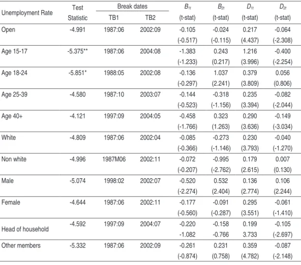
4.1 conventional unit Root tests
As mentioned by Schwert (1989), usual unit root tests, such as ADF, may not be useful if the series contains a moving average component with coefficient close to -1. Therefore, it is important to consider such specification before performing tests for the presence of a unit root in a pure autoregressive process. Column A of Table 3 reports the MA components for all the unemployment series (and their correspond-ing standard errors). As one can see, there is no MA component close to -1 and, therefore, we can move forward and apply the usual unit root tests.
As a benchmark, we start by estimating ADF, PP and KPSS10 unit root tests for all series. The results are reported, respectively, in columns B, C and D of Table 3. Using a 5% level of significance, the ADF estimations cannot reject the unit root hypothesis for all the rates of unemployment and the Phillips-Perron estimations reject the unit root hypothesis for only the Age 15-17 series. Kwiatkowski, Phillips, Schmidt and Shin (1992) see a drawback to testing unit root as a null hypothesis once this null is usually accepted, unless there is strong evidence against it. As a result, the authors propose a unit root test (KPSS) in which the null hypothesis is stationarity against an alternative hypothesis of non-stationarity. The KPSS results indicate that at a level of significance of 1% or 5% there is rejection of the null for all series. Despite the fact that KPSS alternative hypothesis is unit root, this test has power against a fractional unit root (Asikainen, 2003). In this perspective, the KPSS results may be viewed as an evidence in favor of unit root or fractional integration.
However, Baillie et al. (1996) argued that when the KPSS rejects the null hypothesis and the reason is fractional integration, the PP test should reject the unit root null hypothesis, which is the case only for the series Age 15-17. Thus, following Baillie’s
et al. (1996) procedure we would come to the conclusion that the majority of the
series tested have a unit root as there is rejection of the null in all KPSS tests and only one rejection in the PP estimations. But, as mentioned above, ADF and PP-type tests have lower power to make a distinction between unit root and near unit root processes.11 Even though, in this phase, we may come to the conclusion that the series analyzed seem to be I(1), there is still a chance that some confusion can be made between a long memory process and a structural break. And these are our next analysis.
10 See Dickey and Fuller (1979), Phillips and Perron (1988) and Kwiatkowski, Phillips, Schmidt and Shin (1992).
taBlE 3 - unIt Root tEsts
Unemployment Rate Series A B C D
MA(1) (s.e.) ADF PP KPSS
Open 0.199 (0.068) -1.325 -1.473 0.304*
Age 15-17 -0.106 (0.068) -2.576 -4.454* 0.184**
Age 18-24 0.090 (0.066) -1.873 -1.896 0.237*
Age 25-39 0.032 (0.059) -2.298 -2.323 0.308*
Age 40+ 0.027 (0.071) -0.765 -1.340 0.303*
White 0.106 (0.066) -1.556 -2.058 0.298*
Non white 0.086 (0.074) -1.034 -1.507 0.313*
Male 0.187 (0.050) -1.399 -1.550 0.320*
Female 0.108 (0.065) -1.303 -2.023 0.290*
Head of household 0.025 (0.062) -1.149 -1.255 0.342*
Other members 0.136 (0.067) -1.920 -2.019 0.280*
Note: i) ADF, PP and KPSS stand for Augmented Dickey-Fuller, Phillips-Perron and Kwiatkowski-Phillips-Schmidt-Shin, respectively. ii) Estimations with constant and linear trend. iii) ADF’s lagged first differences chosen by the Schwarz Information Criterion. iv) PP and KPSS use Bartlett Kernel with the Newey-West Bandwith. v) *, **, *** mean rejection of H0 at 1%, 5% and 10%.
4.2 unIt Root tEsts WItH stRuctuRal BREaKs
As mentioned previously, in order to examine the order of integration of the unem-ployment series we decided to make use of an endogenous two-break LM unit root test proposed in Lee and Strazicich (2003). Table 4 reports these results. The unit root null hypothesis is rejected for the series related to Age 15-17 (at 10%) and Age 18-24 (at 5%). These two results are different from what was found in the ADF unit root tests. However, the result for Age 15-17 is in line with the PP test. As for the estimations related to Age 18-24, there is some controversy. However, once an omitted broken trend can lead to erroneous conclusions, the unit root tests with structural breaks are more reliable.
Lastly, we notice that the break dates endogenously estimated have some pattern. In general the first break is located either in the end of the 1980s or 1990s. Indeed, in the end of 1980s the unemployment rates decreased, but with the opening of the economy they started to increase again. In addition to that, around 1997 the negative effects of Real Plan over the real variables began to take place. As for the second break, it is usually associated with Lula’s election in 2002.12
taBlE 4 – tWo-BREaK lM tEst
Unemployment Rate Test
Statistic
Break dates B1t B2t D1t D2t
TB1 TB2 (t-stat) (t-stat) (t-stat) (t-stat)
Open -4.991 1987:06 2002:09 -0.105 -0.024 0.217 -0.064
(-0.517) (-0.115) (4.437) (-2.308)
Age 15-17 -5.375** 1987:06 2004:08 -1.383 0.243 1.216 -0.400
(-1.233) (0.217) (3.996) (-2.254)
Age 18-24 -5.851* 1988:05 2002:08 -0.136 1.037 0.379 0.056
(-0.297) (2.241) (3.809) (0.806)
Age 25-39 -4.580 1987:10 2003:07 -0.144 -0.318 0.235 -0.082
(-0.523) (-1.156) (3.394) (-2.044)
Age 40+ -4.121 1997:09 2004:05 -0.458 0.323 0.290 -0.149
(-1.766) (1.263) (3.636) (-3.034)
White -4.809 1987:06 2002:04 -0.085 -0.273 0.230 -0.040
(-0.366) (-1.146) (3.793) (-1.270)
Non white -4.996 1987M06 2002:11 -0.072 -0.995 0.179 0.007
(-0.207) (-2.762) (2.615) (0.130)
Male -5.074 1998:02 2002:07 -0.520 0.532 0.136 0.106
(-2.274) (2.404) (2.774) (2.244)
Female -4.644 1987:06 2002:11 -0.177 -0.091 0.295 -0.061
(-0.560) (-0.287) (3.551) (-1.410)
Head of household -4.592 1997:09 2004:07 -0.220 -0.158 0.199 -0.105
-1.082 -0.766 3.733 (-2.697)
Other members -5.332 1987:06 2002:09 -0.261 0.231 0.359 -0.087
(-0.874) (0.758) (4.782) (-2.148)
Note: * and ** means rejection of H0 at 5% and 10%, respectively.
4.3 aRFIMa Results
We start our analysis by checking the autocorrelations of the series in level and first-differences. However, there is a more precise way to find out whether a series is fractionally integrated or not, which is the point estimation of d, the decay rate. Then, we estimate ARFIMA (0, d, 0) models and report them in Table 5. This is a common procedure as it shows whether ARFIMA estimations without any AR or MA component generate d parameters close to a unit root. In general the value of d is close to 1 (or even larger than 1). The only exception is the series Age 15-17 and this is no surprise as it showed some sign of stationarity in the unit root tests. The null hypothesis d = 0, is rejected for all series, at 5% level. On the other hand, the null hypothesis d = 1 is rejected in four cases: Open, Age 15-17, Male and Other Members. However, only in the case related to the series Age 15-17 the estimated coefficient is lower than 1. This means that, so far, there is strong evidence in favor of persistence caused by long memory or a perfect unit root. But we have to ask whether this procedure is overestimating the parameter d due to the omission of occasional structural breaks.
In order to answer this question we have to check whether the series have structural breaks and whether these breaks influence our results. Based on the break dates selected by Lee and Strazicich’s (2003) unit root test, we employ the procedure due to Granger & Hyung (2004), which is based on the residuals of the follo-wing regression: ut = β'Zt + εt, where Ztcontains the deterministic terms of Lee and Strazicich’s (2003) unit root test (see section 2.2). After that, we estimate an ARFIMA (0, d, 0) model for each series. As we do not use any AR component in the estimation, it is expected that the parameters d be close to or equal to 1 if there is a unit root. If the long memory is caused by the omitted structural breaks, we expect lower values of d.
In summary, except for these two series, it seems that the slow decay of simple au-tocorrelations is due to a pure unit root process. But one result holds for all rates of unemployment examined: all of them are persistent.
taBlE 5
Unemployment Rate
ARFIMA (0,d,0) ARFIMA (0, d, 0) for Residuals
Granger & Hyung’s Procedure
d H0:d=0 H0:d=1 d H0:d=0 H0:d=1
(s.e.) (p.value) (p.value) (s.e.) (p.value) (p.value)
Open 1.213 22.887 4.019 1.080 19.286 1.429
(0.053) (0.000) (0.000) (0.056) (0.000) (0.154)
Age 15-17 0.860 19.545 -3.182 0.711 12.474 -5.070
(0.044) (0.000) (0.002) (0.057) (0.000) (0.000)
Age 18-24 1.069 20.170 1.302 1.005 17.946 0.089
(0.053) (0.000) (0.194) (0.056) (0.000) (0.929)
Age 25-39 1.000 140845 0.000 0.896 15.719 -1.825
(0.000) (0.000) (1.000) (0.057) (0.000) (0.069)
Age 40+ 0.948 18.231 -1.000 0.796 13.724 -3.517
(0.052) (0.000) (0.318) (0.058) (0.000) (0.001)
White 1.089 20.167 1.648 0.991 17.086 -0.155
(0.054) (0.000) (0.100) (0.058) (0.000) (0.877)
Non white 1.058 19.593 1.074 1.009 17.397 0.155
(0.054) (0.000) (0.284) (0.058) (0.000) (0.877)
Male 1.137 19.603 2.362 1.055 18.509 0.965
(0.058) (0.000) (0.019) (0.057) (0.000) (0.335)
Female 1.083 20.434 1.566 0.973 16.776 -0.466
(0.053) (0.000) (0.118) (0.058) (0.000) (0.642)
Head of household 0.998 110.889 -0.222 0.899 15.772 -1.772
(0.009) (0.000) (0.824) (0.057) (0.000) (0.077)
Other members 1.144 22.000 2.769 1.015 18.125 0.268
(0.052) (0.000) (0.006) (0.056) (0.000) (0.789)
Note : The tests for d=0 and d=1 are based on t-distribution.
5 FInal REMaRKs
unemployment rate was analyzed as well as the series disaggregated by gender, age, color and position within the household.
The purpose was to examine whether the unemployment rates followed a perfect unit root or a long memory process. In other words, the aim was to measure the persistence of different labor force groups in the Greater São Paulo Metropolitan Area.
For the period ranging from January 1985 to November 2008, the overall results show that all the unemployment rates analyzed have clear signs of non-stationarity. To be more precise, in general, we did not reject the unit root hypothesis. The ex-ceptions were Age 15-17 and Age 40+, which exhibit long memory (0 < d < 1). In terms of economic policy, these findings mean that all the economic decisions made by the Brazilian policymakers in the past twenty years, as well as changes in real variables, have probably affected the labor forces of São Paulo in a heterogeneous fashion, but in all cases their effects are persistent. Hence, disinflation policies are important and necessary but their negative impacts should also be measured appro-priately and cared for.
REFEREncEs
ARESTIS, P.; MARISCAL, I. Unit roots and structural breaks in OECD unemploy-ment. Economic letters, v. 65, p. 149-156, 1999.
ASIKAINEN, A. long memory and structural breaks in Finnish and swedish party popularity series. University of Helsinki – Department of Economics, 2003. (Discussion Papers n. 586).
BAILLIE, R. T.; CHUNG, C.; TIESLAU, M. A. Analyzing inflation by the frac-tionally integrated Arfima-Garch Model. journal of applied Econometrics, v. 11, n. 1, p. 23-40, 1996.
BAUM, C. F.; BARKOULASB, J. T.; CAGLAYANC, M. Long memory or structural breaks: can either explain nonstationary real exchange rates under the current float? journal of International Financial Markets, Institutions and Money, v. 9, n. 4, p. 359-376, 1999.
______. FRACIRF: stata module to compute impulse response function for fractionally-integrated time-series. Boston College Dept. of Economics, 2000. (statistical software component series n. s414004).
CAMARERO, M.; TAMARIT, C. Hysteresis vs. natural rate of unemployment: new evidence for OECD countries. Economic letters, v. 84, p. 413-417, 2004. CLEMENT, J.; LANASPA, L.; MONTANéS, A. The unemployment structure of
the US States. the Quarterly Review of Economics and Finance, v. 45, p. 848-868, 2005.
DICKEY, D. A.; FULLER, W. A. Distribution of the estimators for auto-regressive time series with a unit root. journal of the american statistical association, v. 74, p. 427-431, 1979.
DIEBOLD, F. X.; RUDEBUSCH, G. D. On the power of Dickey-Fuller tests against fractional alternatives. Economics letters, v. 35, p. 155-160, 1991.
DIEBOLD, F. X.; INOUE, A. Long memory and regime switching. journal of Econometrics, v. 105, p. 131-159, 2001.
DOORNIK, J. A.; OOMS, M. A package for estimating, forecasting and simulating Arfima Models: Arfima package 1.01 for Ox. nuffield college – oxford Discus-sion Paper, 2001.
FRIEDMAN, M. The role of monetary policy. american Economic Review, v. 58, p. 1-17, 1968.
GIL-ALANA, L. A. The persistence of unemployment in the USA and Europe in terms of fractionally ARIMA models. applied Economics, v. 33, p. 1263-1269, 2001a.
______. Measuring unemployment persistence in terms of I(d) statistical models.
applied Economics letters, v. 8, p. 761-763, 2001b.
______; BRIAN HENRY, S. G. Fractional integration and the dynamics of UK unem-ployment. oxford Bulletin of Economics and statistics, v. 65, p. 221-239, 2003. GOMES, F. A. R.; GOMES DA SILVA, C. . Hysteresis versus natural rate of
unem-ployment in Brazil and Chile. applied Economics letters, v. 15, p. 53-56, 2008. ______. Hysteresis versus NAIRU and convergence vs divergence: the behavior of
regional unemployment rates in Brazil. the Quarterly Review of Economics and
Finance, v. 49, p. 308-322, 2009.
GRANGER, C. W. J. Long memory relationships and the aggregation of dynamic models. journal of Econometrics, v. 14, p. 227-238, 1980.
______; Joyeux, R. An introduction to long memory time series and fractional dif-ferencing. journal of time series analysis, v. 1, p. 15-29, 1980.
______.; HYUNG, N. Occasional structural breaks and long memory with an ap-plication to the S&P 500 absolute stock returns. journal of Empirical Finance
11, p. 399-421, 2004.
JAEGER, A.; PARKINSON, M. Some evidence on hysteresis in unemployment rates. European Economic Review, v. 38, p. 329-342, 1994.
KOUSTAS, Z.; VELOCE, W. Unemployment hysteresis in Canada: an approach based on long-memory time series models. applied Economics, v. 28, p. 823-831, 1996.
KWIATKOWSKI, D.; PHILLIPS, P. C. B.; SCHMIDT, P.; SHIN, Y. Testing the null hypothesis of stationarity against the alternative of a unit root: how sure are we that economic time series are non stationary? journal of Econometrics, v. 54, p. 159-178, 1992.
LEE, J.; STRAZICICH, M. C. Break point estimation and spurious rejections with endogenous unit root tests. oxford Bulletin of Economics and statistics, v. 63, p. 535-558, 2001.
______. Minimum LM unit root test with two structural breaks. the Review of Eco-nomics and statistics, v. 85, p. 1082-1089, 2003.
LIMA, E. the naIRu, unemployment and the rate of inflation in Brazil. Rio de Janeiro: IPEA, 2000. (Working Paper 753).
MIKHAIL, O.; EBERWEIN, C. J.; HANDA, J. Testing for persistence in aggre-gate and sectoral Canadian unemployment. applied Economics letters, v. 12, p. 893–898, 2005.
______. Estimating persistence in Canadian unemployment: evidence from a Bayesian ARFIMA. applied Economics, v. 38, p. 1809-1819, 2006.
MITCHELL, W. F. Testing for unit roots and persistence in OECD unemployment.
applied Economics, v. 25, p. 1489–1501, 1993.
NEUDORFER, P.; PICHELMANN, K.; WAGNER, M. Hysteresis, NAIRU and long-term unemployment in Austria. Empirical Economics, v. 15, p. 217-229, 1990.
PERRON, P. The great crash, the oil price shock, and the unit root hypothesis.
Econometrica, v. 57, p. 1361-401, 1989.
______. Further evidence on breaking trend functions in macroeconomic variables.
journal of Econometrics, v. 80, p. 355-385, 1997.
PHELPS, E. Money-wage dynamics and labor-market equilibrium. journal of Political Economy, v. 76, p. 678-711, 1968.
PHILLIPS, P. C. B.; Perron, P. Testing for a Unit Root in Time Series Regression.
Biometrika, v. 75, p. 335-346, 1988.
PORTUGAL, M.; MADALOZZO, R. Um modelo de NAIRU para o Brasil. Revista de Economia Política, v. 20, p. 26-47, 2000.
ROMER, D. advanced macroeconomics. 2nd. ed. New York: McGraw-Hill/Irwin, 2001.
SCHWERT, G. Tests for unit roots: a Monte Carlo investigation. journal of Business and Economic statistics, v. 7, n.2, p. 147-159, 1989.
SONG, F. M.; WU, Y. Hysteresis in unemployment: Evidence from OECD countries.
the Quarterly Review of Economics and Finance, v. 38, p. 181-192, 1998. TOLVI, J. Unemployment persistence of different labor force groups in Finland.
applied Economics letters, v. 10, p. 455-458, 2003.