of Inflation, Inflation Expectations and
Real Interest Rate in Brazil
Cleomar Gomes da Silva
∗
, Maria Carolina da Silva Leme
†
Contents: 1. Introduction; 2. Literature Review; 3. Econometric Methodology; 4. Data; 5. Results; 6. Conclusion.
Keywords: Inflation Persistence, Monetary Policy, Time Series Analysis.
JEL Code: C22, E31, E52.
This paper makes use of Auto-Regressive Fractionally Integrated (AR-FIMA) models, as well as unit root tests with structural breaks, to exa-mine the IPCA (the official inflation rate), inflation expectations, and the real interest rate in Brazil. For the period ranging from July 1999 to December 2010 the results show that the Brazilian inflation can be ta-ken as stationary and mean-reverting, with some degree of persistence. As for inflation expectations, the non-stationarity detected in the frac-tional integration model is due to structural breaks, meaning that they can also be taken as stationary with mean-reversion. Finally, the Selic interest rate shows some sign of non-stationarity, which had already been found in the unit root tests. However, it cannot be characterized by a unit root of a pure form, but as a fractionally integrated process with some long memory.
Este artigo analisa a questão dos graus de persistência do IPCA, da taxa real de juros e das expectativas de inflação no Brasil por intermédio dos Modelos Auto-Regressivos de Integração Fracionada e modelos de raiz unitária com quebra estrutural. O estudo compreende o período de Julho de 1999 a Dezembro de 2010 e seus resultados apontam para uma taxa de inflação brasileira estacionária, com reversão à média e com algum grau de persistência. As expectativas de inflação mostraram características iniciais de não-estacionariedade, sendo isto devido ao problema de quebras estrutu-rais na série. Quando tal problema é resolvido, a série pode ser considerada estacionária e com reversão à média. Finalmente, a taxa real de juros Selic
∗Professor at the Institute of Economics, Federal University of Uberlândia and Adviser to the Secretary of Economic Policy,
Ministry of Finance, Brazil. Disclaimer: The views expressed in this article are those of the author and do not necessarily represent those of the Brazilian Ministry of Finance. E-mail:[email protected]
possui claros sinais de não-estacionariedade, já detectados nos testes de raiz unitária. Contudo, os modelos ARFIMA indicam que a série não segue um processo puro de raiz unitária, mas sim um processo fracionalmente inte-grado e com memória longa.
1. INTRODUCTION
The understanding of the price dynamics is of great importance given that it helps policymakers with the decision making process, by providing accurate approaches to deal with inflation. In other words, when monetary authorities pay attention to the behavior of prices in an economy, they can take preventive measures against possible inflationary pressures, while alleviating costs in terms of inflation tax, GDP, and employment. These issues are related to the inflation persistence phenomenon, which is defined as the implicitly or explicitly predisposition of inflation to converge to the Central Bank’s inflation target.
Regarding interest rates, the investigation of its statistical properties is also essential to the conduct of monetary policy and many studies have tried to determine whether they can be seen asI(0)orI(1). The usual is to consider real interest rates stable in the long term, with mean reversion and no unit root. But they can exhibit long memory and, thus, have a high degree of persistence.
The aim of this paper is to analyze the Brazilian inflation and interest rate persistence based on a univariate approach called Auto-Regressive Fractionally Integrated (ARFIMA), as well as unit root tests with structural breaks. The estimations made take into consideration the following variables: Con-sumer Price Index (IPCA), inflation expectations and the real interest rate. The period under analysis starts in July 1999 and goes up until December 2010. The results show that the Brazilian inflation can be taken as stationary and mean-reverting, with only a small degree of persistence. As for inflation ex-pectations, the non-stationarity detected in the fractional integration model is due to structural breaks, meaning that they can also be taken as stationary with mean-reversion. Finally, the real interest rate shows some sign of non-stationarity, which had already been found in the unit root tests. However, it cannot be characterized by a unit root of a pure form, but as a fractionally integrated process with some long memory.
The article is structured as follows. Section 2 brings the literature review. Section 3 deals with the econometric methodology, and Section 4 describes the data. Section 5 discusses the results, and Section 6 concludes.
2. LITERATURE REVIEW
As far as inflation is concerned, Doornik and Ooms (2004) make use of ARFIMA models to study the British and North American inflationary processes. The latter seems to be stationary, while the former seems to be nonstationarity. Gil-Alana (2005) applies the ARFIMA method for the analysis of the U.S. inflation rate and concludes that the results vary between a persistent and an anti-persistent behavior, according to the specification of the model.
For the Brazilian case, specifically, Cati et al. (1999) study the country’s inflation rate from Jan/1974 and Jun/1993 and show that when statistics that take into account stabilization plans are used, the results show that inflation perturbations were extremely persistent at that period. Campêlo and Cribari-Neto’s (2003) main result indicates the presence of a small inflation inertia in Brazil for the period between Feb/1994 and Feb/2000. Yoon (2003) uses the same data as in Cati et al. (1999) to estimate a unit root test proposed by Ng and Perron (2001) and concludes that the Brazilian inflation rate is nonstationary during the period under analysis.
integrated process. Karanasos et al. (2006) model the dynamics of U.S. ex-post and ex-ante real interest rates and report no unit root in the rates. They also highlight the importance of modeling long memory processes. Caporale and Gil-Alana (2009) study the degree of persistence of the U.S. and state that the fractional estimations seem to be very sensitive to the specification of the model.
Gil-Alana (2003) estimates the behavior of short run interest rates in Singapore, Thailand, Malaysia, South Korea, the Philippines. The author shows that there is mean reversion for the Thai and Singa-porean interest rates, whilst the results for the other countries are less conclusive. Iglesias and Phillips (2005) use ARFIMA models to study the behavior of short-term interest rates of six European countries and find that the Swiss series seems to beI(1). Couchman et al. (2006) examine the long memory properties of real interest rates for 16 countries. The majority of them have long-memory parameters between zero and one. Candelon and Gil-Alana (2006) analyze the short-run interest rates in Singapore, Thailand, Mexico, Malaysia, the Phillipines, and Korea by means of fractional integration. The authors find that in only the two first ones the nominal interest rates are mean-reverting.
3. ECONOMETRIC METHODOLOGY
3.1. ARFIMA models
The analysis of inflation persistence can be performed by the use of several unit root tests found in the literature. But they assume only integer values, i.e. I(0) if stationary andI(1) if not. The ARFIMA (Autoregressive Fractionally Integrated Moving Average) methodology, as defined by Granger and Joyeux (1980) e Hosking (1981), generalizes ARIMA models(p, d, q)and allows for fractional values of the order of integration ‘d’ between 0 and 1. In other words, the flexibility of the ARFIMA models increases the acuity of the analysis by better defining degree of persistence of each series – a step forward in relation to the rigid unit root tests. Moreover, the ARFIMA models improve the low power behavior of the unit root test and are also capable of modeling the dynamics of short and long run inflationary processes through the estimation of impulse response functions.
A basic ARIMA model(p, q)can be written in the following way:
yt=c+α1yt−1+· · ·+αpyt−p+ut+β1ut−1+· · ·+βqut−q, t= 1,· · ·,T (1)
where ‘α’ e ‘β’ are coefficients and ‘u’ is the error term withut=N ID[0, σ 2
]. In lag operator form:
1−α1L−α2L2
− · · · −αpLpyt=c+ 1 +β1L+β2L 2
+· · ·+βqLqut (2)
Dividing both sides by the LHS term:1
yt=µ+ Φ(L)ut (3)
where:
Φ(L) = (1 +β1L+β2L 2
+· · ·+βqLq)
(1−α1L−α2L2− · · · −αpLp)
∞
X
j=0
|Φj|<∞
µ= c
(1−α1−α2− · · · −αp)
An integrated process of order ‘d’ can have the following representation:
(1−L)dy
t= Φ(L)ut (4)
with P∞
j=0|Φj| < ∞. Usually, it is assumed ‘d ′
= 1, or that the first difference of the series is stationary.
However, these noninteger values of ‘d’ can be of great use. Consider the MA representation(∞)
in (2). If ‘d′
>0.5, the reverse of the operator(1−L)−dexists. That can be seen by multiplying both sides of the first equation by(1−L)−d. The result is as follows:
yt= (1−L) −d
Φ(L)ut (5)
The operator(1−L)−dcan be represented by the following filter:
(1−L)−d= 1 +dL+ (1/2!)(d+ 1)dL2
+ (1/3!)(d+ 2)(d+ 1)dL3
+· · ·= ∞
X
j=0
λjLj (6)
whereλ0≡1and:
λj = (1/j!)(d+j−1)(d+j−2)(d+j−3)· · ·(d+ 1)(d) (7)
It can be demonstrated2that, ifd <1, λ
jcan be approximated for largejby:
λj ∼= (j+ 1)d −1
(8)
Therefore, an MA representation(∞)in which the coefficient of the impulse responseλjbehaves for largejlike(j+ 1)d−1
can be defined as:
yt= (1−L) −d
ut=λ0ut+λ0ut−1+λ0ut−2+· · · (9)
The autocorrelations of the stationary ARIMA series can have an exponential decrease, while frac-tionally integrated series have hyperbolic decreases. In other words, while the coefficients of an ARIMA stationary impulse-response disappear geometrically, the processes of equation (7) imply a gradual and slower decay. That is why fractionally integrated series are also denominated long memory time series (Hamilton, 1994).
In addition to that, the sequence of the limiting MA coefficients, given in equation (7), can be shown to besquare-summableso long as‘d′
<0.5:
∞
X
j=0 λ2
j <∞ for d <0.5 (10)
Thus, ford <0.5, the aim is to difference the process before performing the description presented in equation (3) (Hamilton, 1994).
As mentioned above, low levels of ‘d’ characterize weak persistence in the ARFIMA models, while in the traditional unit root models these are nonexistent persistence. On the other hand, high levels of ‘d’ are considered persistent with reversion to the mean, whereas in the traditional unit root tests such persistence exists but with no reversion to the mean. In sum, the ARFIMA models have the following rules:
1) if0 ≥ ‘d′
≤ 0.5the series is stationary with reversion to the mean and it is a process of long memory;
2) if0.5<‘d′
≤1, the series is non stationary but still mean reverting;
3) if‘d′
≥1, the series is non stationary and does not have mean reversion (Gil-Alana, 2001);
4) if−0.5<‘d′
<0, the process is called over-differenced.
Three estimation methods of the ARFIMA models are commonly used: Exact Maximum Likelihood (EML), Modified Profile Likelihood (MPL), and Nonlinear Least Squares (NLS).3 By definition, both EML
and MPL impose−1 <‘d′
< 0.5. If the model includes regressor variables and the sample is small, the MPL is preferred over the EML. The NLS methodology allows for‘d′
>−0.5and can be used in the estimation of nonstationary series (Baillie et al., 1996).
Given that the series analyzed seem to be nonstationary, the EML methodology does not apply because it is seriously biased downwards for ‘d’ values close to 0.5 and greater than 0.5. Therefore, we make use of the NLS methodology, which does not present these usual biases. The NLS estimator is based on the maximization of the following likelihood function:
ℓN(d,Φ,Θ) =−
1 2log
1 T
N
X
i=1 ˜ et
!
(11)
where the residuals˜etare obtained by applying the ARFIMA(p, d, q)model to theutand the vectorsΦ andΘrepresent the autoregressive parameters ‘p’ and the moving average ‘q’ respectively.
3.2. Structural breaks
Besides examining whether the series have long memory properties, we have to check if they have structural breaks. As mentioned, this is important once one may conclude that a series has a long memory process when it is actually influenced by structural breaks.
In order to examine the order of integration of the series we first apply unit root tests, such as ADF and KPSS. However, since Perron (1989), it is well known that ADF tests can fail to reject a false unit root due to misspecification of the deterministic trend. In fact, Perron (1989, 1997) and Zivot and Andrews (1992) extend the ADF test considering an exogenous and an endogenous break to avoid this problem. But these types of tests also have some drawbacks once they derive their critical values assuming no break(s) under the null hypothesis, which lead to a spurious rejection of the null hypothesis in the presence of a unit root with breaks (Lee and Strazicich, 2001).
Therefore, we decided to make use of an endogenous two-break LM unit root test proposed in Lee and Strazicich (2003). In contrast to the ADF-type tests, the properties of these LM tests are unaffected by breaks under the null. According to the LM (score) principle, a unit root test statistic can be obtained from the following regression:
△ut=g ′
△Zt+φS˜t−1+ k
X
i=1
γi△S˜t−i+εt (12)
where:
i) S˜tis a de-trended series such thatS˜t=ut−ψ˜x−Ztδ,t˜ = 2, . . . ,T;
ii) δ˜is a vector of coefficients in the regression of △uton△Ztand ψ˜x = u1−Z1δ˜, whereZtis defined below;
iii) u1andZ1are the first observations ofutandZt, respectively;
iv) △S˜t−i(wherei= 1, . . . ,k) terms are included as necessary to correct for serial correlation;
v) Ztis a vector of exogenous variables defined by the data generating process.
Considering two changes in level and trend,Ztis described by[1,t,D1t,D2t,DT ∗ 1t,DT
∗ 2t]
′
, whereDjt=
1fort≥TBj+ 1,j= 1,2, and zero otherwise,DT ∗
jt=tfort≥TBj+ 1,j= 1,2, and zero otherwise, andTBjstands for the time period of the breaks. Note that the test regression (12) involves△Ztinstead ofZtso that△Ztbecomes[1,B1t,B2t,D1t,D2t]′, whereBjt=△DjtandDjt=△DTjt∗,j= 1,2.
The unit root null hypothesis is described in equation (12) byφ= 0and the test statistics is defined asρ˜=T.φ˜. For the null hypothesis ,(φ= 0),τ˜=t-statistic. To endogenously determine the location of the two breaks(λj=TBj/T,j= 1,2)we use theLMτ=Infλτ˜(λ). As in Lee and Strazicich (2003), we use critical values that correspond to the location of the breaks,(λj =TBj/T,j= 1,2).
4. DATA
The period under analysis ranges from July 1999 to December 2010. The series investigated are the 12-month IPCA, the real (Selic) interest rate and the 12-month ahead inflation expectations (from July 2001 to December 2010).
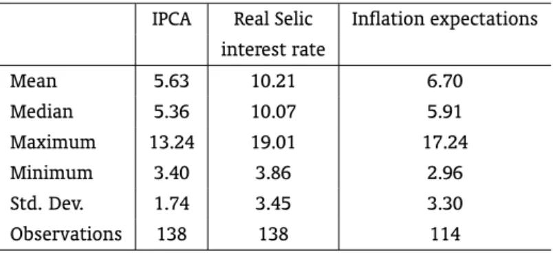
Table 1 presents the descriptive statistics of the data. One can see that the average inflation rate (IPCA) in Brazil is 5.63%, meaning that it is above the central inflation target (4.5%). The average inflation expectation is higher (6.70%) and the average real Selic interest rate is even higher (10,21%). The medians also follow the same pattern and the standard deviations related to the Selic rate and inflation expectations are close to each other and twice the value of IPCA. The maximums usually refer to a period between the second semester 2002 and first semester 2003.
Table 1: Descriptive statistics (%)
IPCA Real Selic Inflation expectations interest rate
Mean 5.63 10.21 6.70
Median 5.36 10.07 5.91
Maximum 13.24 19.01 17.24
Minimum 3.40 3.86 2.96
Std. Dev. 1.74 3.45 3.30
Observations 138 138 114
Source: IBGE.
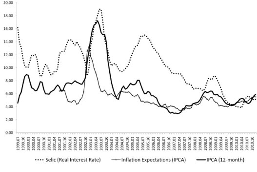
Figure 1 provides a better understanding of the descriptive analysis, mainly in relation to the max-imums reported in Table 1. Bresser-Pereira and Gomes da Silva (2008) point out that the Brazilian economy was hit by a series of unfavorable shocks, in 2001, such as the energy crisis, Argentina’s crisis and the terrorist attacks in the USA. All of these caused strong exchange rate depreciation as well as in-creases in monitored prices. The monetary authorities tried to limit the propagation of the disturbances faced by the economy and started working with a more restrictive monetary policy. Nevertheless, the inflation rate reached 7.7% in 2001, meaning that the target was breached.
coun-Figure 1: IPCA, Selic Interest Rate and Inflation Expectations (%) – (Jul/1999-Dec/2010) 6,00 8,00 10,00 12,00 14,00 16,00 18,00 20,00 0,00 2,00 4,00 1 9 9 9 .0 7 1 9 9 9 .1 0 2 0 0 0 .0 1 2 0 0 0 .0 4 2 0 0 0 .0 7 2 0 0 0 .1 0 2 0 0 1 .0 1 2 0 0 1 .0 4 2 0 0 1 .0 7 2 0 0 1 .1 0 2 0 0 2 .0 1 2 0 0 2 .0 4 2 0 0 2 .0 7 2 0 0 2 .1 0 2 0 0 3 .0 1 2 0 0 3 .0 4 2 0 0 3 .0 7 2 0 0 3 .1 0 2 0 0 4 .0 1 2 0 0 4 .0 4 2 0 0 4 .0 7 2 0 0 4 .1 0 2 0 0 5 .0 1 2 0 0 5 .0 4 2 0 0 5 .0 7 2 0 0 5 .1 0 2 0 0 6 .0 1 2 0 0 6 .0 4 2 0 0 6 .0 7 2 0 0 6 .1 0 2 0 0 7 .0 1 2 0 0 7 .0 4 2 0 0 7 .0 7 2 0 0 7 .1 0 2 0 0 8 .0 1 2 0 0 8 .0 4 2 0 0 8 .0 7 2 0 0 8 .1 0 2 0 0 9 .0 1 2 0 0 9 .0 4 2 0 0 9 .0 7 2 0 0 9 .1 0 2 0 1 0 .0 1 2 0 1 0 .0 4 2 0 1 0 .0 7 2 0 1 0 .1 0
Selic (Real Interest Rate) Inflation Expectations (IPCA) IPCA (12-month)
Note: Inflation Expectations (from July 2001 to December 2010) Source: IPEADATA
try’s fundamentals fled the country, leading to more depreciation of the exchange rate and characteriz-ing the so-called fiscal dominance (Bresser-Pereira and Nakano, 2002). Under that condition, respondcharacteriz-ing to higher inflation with interest rate increases leads to a real exchange rate depreciation and, conse-quently, to a further increase in inflation. If this is the case, the right instrument to lower inflation would be fiscal (not monetary) policy (Favero and Giavazzi, 2005).
After the presidential election, in October 2002, the new government planned a primary surplus target and announced a reform of the social security system. There was a decrease in the probability of default, an appreciation of the Real, and a decrease in inflation (Blanchard, 2005).
5. RESULTS
5.1. Conventional unit root tests
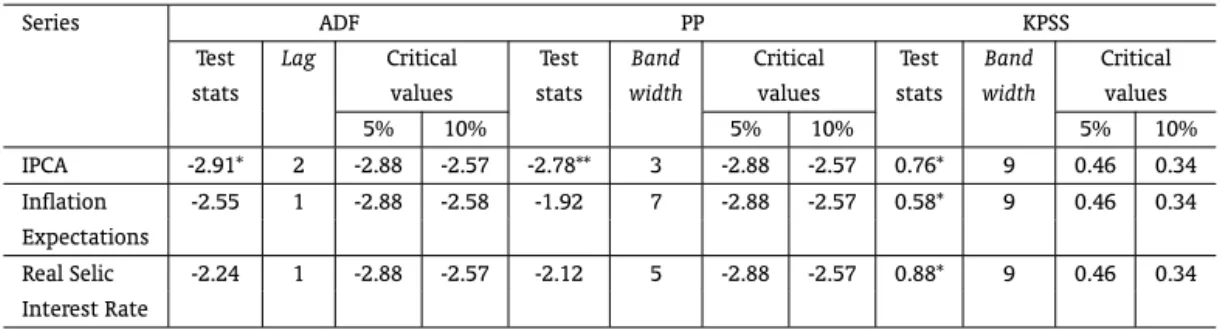
As a benchmark, we start by estimating ADF and KPSS4unit root tests for all series (Table 2). At
5% level of significance, the ADF estimations reject the unit root hypothesis for the IPCA, but not for
the inflation expectations and the real Selic interest rate. On the other hand, the KPSS results report rejection of the null for all series (at 5%), indicating non-stationarity.
However, Baillie et al. (1996) argued that if the KPSS rejects the null hypothesis and the reason is fractional integration, the Phillips-Perron (PP) test should reject the unit root null hypothesis, which is the case only for the IPCA. Therefore, following the authors’ procedure one would come to the conclu-sion that the majority of the series tested have a unit root, as there is rejection of the null in all KPSS tests and only one rejection in the PP estimations. But, as mentioned previously, ADF and PP-type tests have lower power to make a distinction between unit root and near unit root processes.5 There is still a chance of confusion between a long memory process and a structural break, which will be checked further on.
Table 2: Conventional unit root tests
Series ADF PP KPSS
Test Lag Critical Test Band Critical Test Band Critical
stats values stats width values stats width values
5% 10% 5% 10% 5% 10%
IPCA -2.91* 2 -2.88 -2.57 -2.78** 3 -2.88 -2.57 0.76* 9 0.46 0.34
Inflation -2.55 1 -2.88 -2.58 -1.92 7 -2.88 -2.57 0.58* 9 0.46 0.34
Expectations
Real Selic -2.24 1 -2.88 -2.57 -2.12 5 -2.88 -2.57 0.88* 9 0.46 0.34
Interest Rate
Note: Estimations with constant only. *, ** mean rejection of the null at 5% and 10%.
5.2. Unit root tests with structural breaks
In order to examine the order of integration of the series, taking into consideration the possibility of breaks, we make use of an endogenous two-break LM unit root test proposed in Lee and Strazicich (2003). Table 3 lists the two breakpoints for the three series, with their significance and timing. The unit root null hypothesis is rejected for the inflation expectations and IPCA, but not for the real interest rate. This sheds some more light on the conventional unit root tests (Table 2), as they showed mixed results, mainly for the IPCA and inflation expectations. However, it seems that the Selic rate has some sign of non-stationarity, which might be controversial and needs more research related to the possibility of a long memory process.
5.3. ARFIMA Results
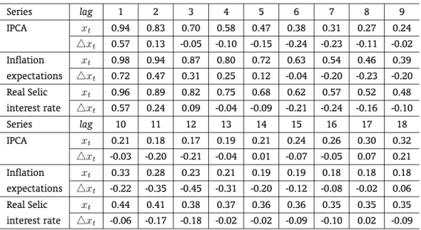
Before analyzing the ARFIMA results, it is important to look at the autocorrelation of the series (Table 4). In levels, the values begin at 0.98 or 0.99 and then decay very slowly, which is consistent with a non-stationary process. As for the first differences, when a series is fractionally integrated and ‘d′
<1, the first difference operator causes overdifference of the series. In this case, we should expect negative values in the first autocorrelations. Table 4 shows that the first negative sign for the IPCA is on the third lag, for the inflation expectations on the sixth lag and for the Selic interest rate on the fourth lag.
Table 3: Two break unit root LM test
Series Test Break dates 1st break 2nd break
statistic 1st break 2nd break B1t D1t B2t D2t [t-stat] [t-stat] [t-stat] [t-stat] IPCA -6.16* 2002:09 2004:06 -0.32 0.38 0.47 -0.82
[-0.75] [0.90] [3.10] [-4.59] Inflation -6.52* 2003:03 2008:01 1.54 -0.07 -0.25 0.54
expectations [3.39] [-0.19] [-2.42] [5.26]
Real Selic -5.11 2003:07 2005:04 0.67 0.31 -1.06 0.53
interest rate [0.91] [0.43] [-4.48] [2.71]
Note: * and ** means rejection of H0 at 5% and 10%, respectively. Critical values from Lee and Strazicich (2003).
Table 4: Autocorrelations – Series in level and in first difference
Series lag 1 2 3 4 5 6 7 8 9
IPCA xt 0.94 0.83 0.70 0.58 0.47 0.38 0.31 0.27 0.24
△xt 0.57 0.13 -0.05 -0.10 -0.15 -0.24 -0.23 -0.11 -0.02 Inflation xt 0.98 0.94 0.87 0.80 0.72 0.63 0.54 0.46 0.39 expectations △xt 0.72 0.47 0.31 0.25 0.12 -0.04 -0.20 -0.23 -0.20 Real Selic xt 0.96 0.89 0.82 0.75 0.68 0.62 0.57 0.52 0.48 interest rate △xt 0.57 0.24 0.09 -0.04 -0.09 -0.21 -0.24 -0.16 -0.10
Series lag 10 11 12 13 14 15 16 17 18
IPCA xt 0.21 0.18 0.17 0.19 0.21 0.24 0.26 0.30 0.32
For the ARFIMA(p, d, q)models estimations we follow the standard procedure of using Autore-gressive (AR) and Moving Average (MA) representations up to the third lag, generating 16 different estimations for each model. After that, we use the Schwarz Information Criterion to select the best model for each of the series.
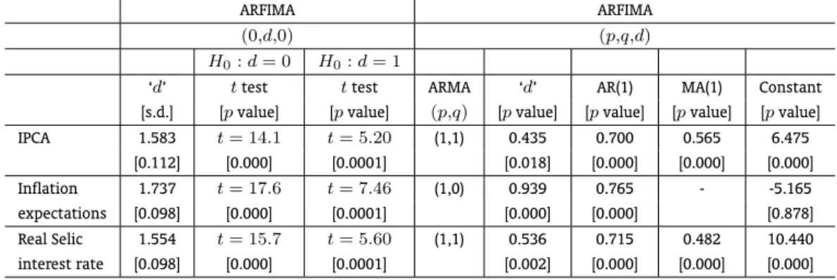
But before selecting the best model, we can look at the ARFIMA(0, d,0)estimations, without any AR or MA component, to see if they generate ‘d’ parameters close to a unit root or not. Table 5 reports that in all three cases the values of ‘d’ are larger than 1. The null hypothesis ‘d′
= 0is rejected for all series, at 5% level, as well as the null hypothesis ‘d′
= 1. This means that, so far, there is strong evidence in favor of persistence caused by long memory or perfect unit root.
As for the models selected, Table 5 shows that for the IPCA the best estimation is an ARFIMA (1, 0.435, 1), i.e., stationary and with reversion to the mean. We can compare this result with those found in the unit root tests in order to detect gains obtained by using long memory models. The fractional result goes along with the ones reported for the ADF tests and for the LM unit root test. As a comparison, Doornik and Ooms (2004) found a parameter ‘d′
= 0.25for the American case and0.47<‘d′ <0.59
for the British case. Gil-Alana (2005) found ‘d′
= 0.25for the American case.
For the Selic real interest rate the best model selected is an ARFIMA (1, 0.536, 1). This characterizes the series as nonstationary, which is in line with all the unit root tests performed. But the difference is the mean-reversion in the long run.
For the Inflation Expectations, the estimation points toward an ARFIMA (1, 0.939, 0) as the most ap-propriate model, indicating nonstationarity, as detected by the unit root tests (see Table 3), but reverting to the mean in the long run. This is an unexpected result, given that, lately, inflation expectations have converged to the values set by the targets. But we know that the series was strongly affected by sev-eral shocks, contributing to its high persistence (see Figure 1). This can be seen when we look at the two-break unit root LM test, which has already shown stationarity in the series. Further analysis must be conducted to determine the influence of breaks on the results.
Table 5: ARFIMA estimations
ARFIMA ARFIMA
(0,d,0) (p,q,d)
H0:d= 0 H0:d= 1
‘d’ ttest ttest ARMA ‘d’ AR(1) MA(1) Constant
[s.d.] [pvalue] [pvalue] (p,q) [pvalue] [pvalue] [pvalue] [pvalue]
IPCA 1.583 t= 14.1 t= 5.20 (1,1) 0.435 0.700 0.565 6.475
[0.112] [0.000] [0.0001] [0.018] [0.000] [0.000] [0.000]
Inflation 1.737 t= 17.6 t= 7.46 (1,0) 0.939 0.765 - -5.165
expectations [0.098] [0.000] [0.0001] [0.000] [0.000] [0.878]
Real Selic 1.554 t= 15.7 t= 5.60 (1,1) 0.536 0.715 0.482 10.440
interest rate [0.098] [0.000] [0.0001] [0.002] [0.000] [0.000] [0.000]
5.4. Fractional Integration and Structural Breaks
Going one step ahead, there is still the possibility of confusion between long memory and struc-tural breaks, and this can influence our results. Therefore, we have to ask whether the usual ARFIMA regression is overestimating the parameter ‘d’ due to the omission of occasional structural breaks.
yt=β ′
Zt+ξt (13)
where ‘y’ represents one of the series to be analyzed andZtcontains the corresponding deterministic terms of Lee and Strazicich’s (2003) unit root test. After that, we estimate other ARFIMA models. If this method is able to generate lower ‘d’ values, then the long memory process might well be due to the breaks.
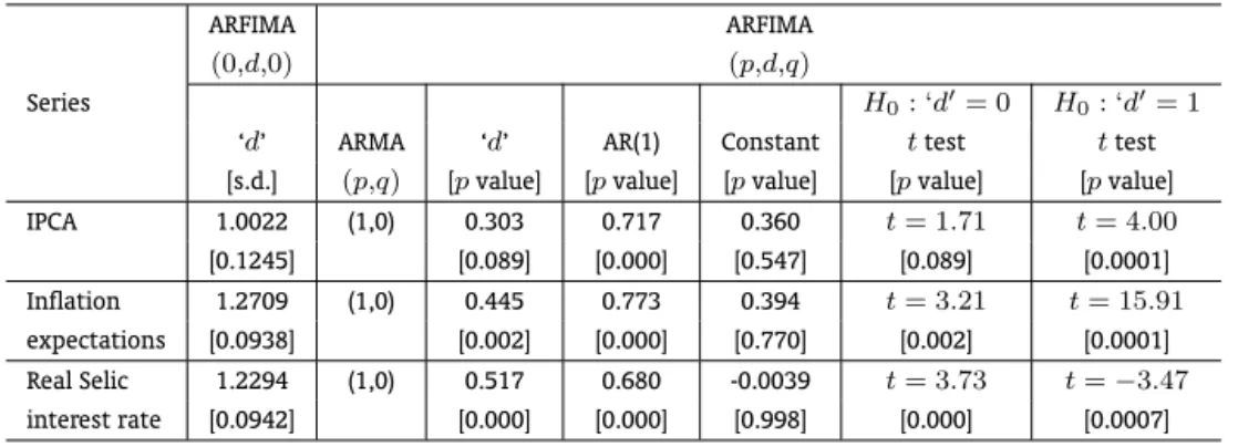
Table 6 reports the results of the models based on the residuals related to Granger and Hyung’s (2004) procedure. First of all, the ARFIMA (0, d, 0) regressions, without any AR or MA component, show that the point estimation of ‘d’ decreases for all series. Thus, it seems that the omission of occasional breaks in the previous analysis leads to overestimated coefficients. But there is some sign of non-stationarity and no mean reversion.
Table 6 also shows that for the IPCA-Residuals the best estimation is an ARFIMA (1, 0.303, 0), which is quite in line with the values found in the Table 5 and with the unit root tests. The null hypothesis ‘d′
= 0cannot be rejected, at 5% level, but it is rejected for ‘d′ = 1.
For the Inflation Expectations the model chosen is an ARFIMA (1, 0.445, 0), which makes the series stationary and mean reverting, as opposed to what was detected previously. Therefore, it seems that the non-stationarity found in the previous test was due to structural breaks. The null hypothesis ‘d′
= 0
is rejected, at 5% level, as well as the null hypothesis ‘d′ = 1.
For the Selic Interest Rate the best model is an ARFIMA (1, 0.517, 0). This is interesting once the ‘d’ parameter found is close to the one reported on Table 5. At 5% level, the null hypothesis ‘d′
= 0is rejected, as well as the null hypothesis ‘d′
= 1. It means that even when breaks are accounted for, we still find that the real interest rate in Brazil has a long memory, though mean reverting in the long run.
Table 6: ARFIMA(0, d,0)for Residuals – Granger & Hyung’s procedure
ARFIMA ARFIMA
(0,d,0) (p,d,q)
Series H0: ‘d′= 0 H0: ‘d′= 1
‘d’ ARMA ‘d’ AR(1) Constant ttest ttest
[s.d.] (p,q) [pvalue] [pvalue] [pvalue] [pvalue] [pvalue]
IPCA 1.0022 (1,0) 0.303 0.717 0.360 t= 1.71 t= 4.00
[0.1245] [0.089] [0.000] [0.547] [0.089] [0.0001]
Inflation 1.2709 (1,0) 0.445 0.773 0.394 t= 3.21 t= 15.91
expectations [0.0938] [0.002] [0.000] [0.770] [0.002] [0.0001]
Real Selic 1.2294 (1,0) 0.517 0.680 -0.0039 t= 3.73 t=−3.47
interest rate [0.0942] [0.000] [0.000] [0.998] [0.000] [0.0007]
6. CONCLUSION
This article aimed at analyzing inflation persistence in Brazil, as well as the degree of persistence in inflation expectations and in the Selic real interest rate, for the period ranging from July 1999 to December 2010. As far as econometric methodology was concerned, we made use of Auto-Regressive Fractionally Integrated (ARFIMA) models, and unit root tests with structural breaks as well.
showing that part of the persistence is due to structural breaks observed in the series in the period analyzed.
As for inflation expectations, they are also stationary with mean-reversion. But this result was only reached after testing the residuals of the unit root tests with structural breaks, which were responsible for the high degree of persistence in the series detected in the initial fractional integration estimations. Finally, the Selic interest rate shows signs of non-stationarity, which was found initially in the unit root tests. The ARFIMA models provided results reporting that the Brazilian real interest rate series is not a unit root of a pure form, but fractionally integrated and, therefore, persistent. The analysis of the residuals of the unit root tests with structural breaks makes no difference in the ’d’ parameter estimated, meaning that the degree of persistence found cannot be blamed on structural breaks. But the parameter calculated is close to stationarity.
Thus, one can conclude that inertial inflation in Brazil has been controlled and it is going towards international levels. On the other hand, the real interest rate seem to be highly persistent along time, even though it is close to stationarity.
BIBLIOGRAPHY
Baillie, R. T., Chung, C., & Tieslau, M. A. (1996). Analyzing inflation by the fractionally integrated Arfima-Garch model.Journal of Applied Econometrics, 11(1):23–40.
Blanchard, O. (2005). Fiscal dominance and inflation targeting: Lessons from Brazil. In Giavazzi, F., Goldfajn, I., & Herrera, S., editors,Inflation Targeting, Debt and the Brazilian Experience, pages 49–80. MIT Press, Cambridge, MA.
Bresser-Pereira, L. C. & Gomes da Silva, C. (2008). Inflation targeting in Brazil: A Keynesian approach. In Wray, L. R. & Forstater, M., editors,Keynes and Macroeconomics After 70 Years, pages 176–195. Edward Elgar, Cheltenham, UK.
Bresser-Pereira, L. C. & Nakano, Y. (2002). Uma estratégia de desenvolvimento com estabilidade. Revista
de Economia Política, 22:146–180.
Campêlo, A. K. & Cribari-Neto, F. (2003). Inflation inertia and inliers: The case of Brazil.Revista Brasileira
de Economia, 57(4):713–739.
Candelon, B. & Gil-Alana, L. A. (2006). Mean reversion of short-run interest rates in emerging countries.
Review of International Economics, 14(1):119–135.
Caporale, M. G. & Gil-Alana, L. A. (2009). Persistence in US interest rates: Is it stable over time?
Quanti-tative and QualiQuanti-tative Analysis in Social Sciences, 3(1):63–77.
Cati, R., Garcia, M., & Perron, P. (1999). Unit roots in the presence of abrupt governmental interventions with an application to Brazilian data.Journal of Applied Econometrics, 14:27–56.
Couchman, J., Gounder, R., & Su, J. J. (2006). Long memory properties of real interest rates for 16 countries. Applied Financial Economics Letters, 2:25–30.
Dickey, D. A. & Fuller, W. A. (1979). Distribution of the estimators for autoregressive time series with a unit root. Journal of the American Statistical Association, 74:427–431.
Diebold, F. X. & Rudebusch, G. D. (1991). On the power of Dickey-fuller tests against fractional alterna-tives.Economics Letters, 35(2):155–160.
Doornik, J. A. & Ooms, M. (2004). Inference and forecasting for ARFIMA models, with an application to US and UK inflation.Studies in Nonlinear Dynamics and Econometrics, 8(2). Article 14.
Favero, C. A. & Giavazzi, F. (2005). Inflation targeting and debt: Lessons from Brazil. In Giavazzi, F., Goldfajn, I., & Herrera, S., editors,Inflation Targeting, Debt and the Brazilian Experience, 1999 to 2003, pages 85–108. MIT Press, Cambridge, MA.
Gil-Alana, L. A. (2001). The persistence of unemployment in the USA and Europe in terms of fractionally ARFIMA models.Applied Economics, 33:1263–9.
Gil-Alana, L. A. (2002). A mean shift break in the US interest rate.Economics Letters, 77(3):357–363.
Gil-Alana, L. A. (2003). Long memory in the interest rates in some Asian countries. Journal International
Advances in Economic Research, 9(4):257–267.
Gil-Alana, L. A. (2004). Long memory in the US interest rate. International Review of Financial Analysis, 13:265–276.
Gil-Alana, L. A. (2005). Testing and forecasting the degree of integration in the US inflation rate.Journal
of Forecasting, 24:173–187.
Granger, C. & Hyung, N. (2004). Occasional structural breaks and long memory with an application to the S&P 500 absolute stock returns. Journal of Empirical Finance, 11:399–421.
Granger, C. & Joyeux, R. (1980). An introduction to long memory time series and fractional differencing.
Journal of Time Series Analysis, 1:15–29.
Hamilton, J. (1994). Time Series Analysis. Princeton University Press, Princeton, NJ.
Hosking, J. R. M. (1981). Modeling persistence in hydrological time series using fractional differencing.
Water Resources Research, 20:1898–908.
Iglesias, E. M. & Phillips, G. D. A. (2005). Analyzing one-month Euro-market interest rates by fractionally integrated models.Applied Financial Economics, 15(2):95–106.
Karanasos, M., Sekioua, S., & Zeng, N. (2006). On the order of integration of monthly US ante and ex-post real interest rates: New evidence from over a century of data. Economics Letters, 90(2):163–169.
Kwiatkowski, D., Phillips, P. C. B., Schmidt, P., & Shin, Y. (1992). Testing the null hypothesis of stationarity against the alternative of a unit root: How sure are we that economic time series are non-stationary?
Journal of Econometrics, 54:159–178.
Lai, K. S. (1997). Long term persistence in real interest rates. Some evidence of a fractional unit root.
International Journal of Finance and Economics, 2:225–235.
Lee, J. & Strazicich, M. C. (2001). Break point estimation and spurious rejections with endogenous unit root tests. Oxford Bulletin of Economics and Statistics, 63:535–558.
Lee, J. & Strazicich, M. C. (2003). Minimum LM unit root test with two structural breaks. The Review of
Economics and Statistics, 85:1082–1089.
Ng, S. & Perron, P. (2001). Lag length selection and the construction of unit root tests with good size and power.Econometrica, 69:1519–54.
Perron, P. (1997). Further evidence on breaking trend functions in macroeconomic variables. Journal of
Econometrics, 80:355–385.
Phillips, P. C. B. & Perron, P. (1988). Testing for a unit root in time series regression.Biometrika, 75:335– 346.
Tsay, W. (2000). Long memory story of the real interest rate. Economics Letters, 67(3):325–330.
Yoon, G. (2003). The time series behavior of Brazilian inflation rate: New evidence from unit root tests with good size and power. Applied Economics Letters, 10:627–631.