Across Brazilian States
∗
Luiz Renato Lima
†
, Hilton Hostalácio Notini
‡
, Fábio Augusto Reis
Gomes
§
Contents: 1. Introduction; 2. ARFIMA Models and the Convergence Hypothesis; 3. Econometric Methodology ; 4. Results; 5. Conclusion.
Keywords: Growth Model, Stochastic Convergence, Long Memory, Brazil. JEL Code: C22, O49, O54, R11.
The aim of this paper is to analyze the convergence hypothesis across Brazilian States in a 60 year period (1947-2006). In order to test the existence of income convergence, the order of integration of the in-come differences between each State and São Paulo is examined. The time series approach does not include any covariate and, as a result, it can be viewed as an unconditional test. São Paulo is the richest State and for this reason is used as a benchmark. First of all, we employed the conventional unit root tests, finding evidence against the conver-gence hypothesis. However, given the lack of power of unit root tests, especially when the rate of convergence is very low, we used ARFIMA models, which is also theoretically more appropriate (Michelacci e Zaf-faroni, 2000). Even so, the estimation results of the ARFIMA models cast doubts on the convergence hypothesis.
O objetivo deste trabalho é analisar a hipótese de convergência entre os estados brasileiros, considerando um período de 60 anos (1947-2006). Para testar a existência de convergência de renda, foi examinada a ordem de in-tegração das séries da diferença de renda entre cada estado e o estado de São Paulo. Esta abordagem de séries temporais não inclui nenhuma regres-sor na análise e, como consequência, pode ser vista como um teste incondi-cional. São Paulo é o estado mais rico e, por isso, é usado como referência. Primeiramente, foram empregados os testes de raiz unitária tradicionais, sendo encontrada evidência contra a hipótese de convergência. No entanto,
∗The authors would like to express their appreciation to the participants in the III Economics Seminar in Belo Horizonte and IV
CAEN-EPGE Seminar of Public Policy and Economic Growth for helpful comments. All the remaining errors are ours.
†Department of Economics, University of Tennessee. E-mail:[email protected]
‡Agência Nacional de Aviação Civil (ANAC) and Getulio Vargas Foundation-RJ. E-mail:[email protected]
dado o baixo poder dos testes de raiz unitária, especialmente quando a taxa de convergência é muito baixa, usamos modelos ARFIMA, que também são teoricamente mais adequados (Michelacci e Zaffaroni, 2000). Mesmo assim, os resultados da estimação dos modelos ARFIMA lançam dúvidas sobre a hipótese de convergência.
1. INTRODUCTION
According to the neoclassical growth model, economies converge to their own steady state, regard-less of their initial per capita output. Furthermore, the speed of convergence is inversely related to the gap between current income and its steady state value (Solow, 1956). If the parameters that character-ize the steady states of a group of countries are identical, then their difference lies in their initial level of capital and poor economies should grow faster because they are further away from the steady state. This proposition is named absolute convergence. On the other hand, one can allow for heterogeneity across economies by dropping the assumption that all economies have the same steady state. In this case, economies are convergent only after controlling for their steady states. This proposition is known as conditional convergence, and it gave rise to an immense empirical literature that analyzes its suit-ability. Initially, the literature focused on country comparisons using cross-section data; however, some authors also explored the time series dimension.
In the cross-section approach, a negative correlation between income growth rates and initial in-come is interpreted as evidence of unconditionalβ-convergence, where unconditional means that coun-tries’ characteristics are not taken into account. The conditionalβ-convergence analysis requires the inclusion of conditioning variables, like investment rate and population growth, in order to interpret the convergence rate as a measure of conditional convergence (Durlauf, 2001). In this context, one of the most generally accepted results is that, while there is evidence of unconditional convergence inside homogenous group of countries or regions, only the conditional convergence hypothesis holds when examining broad groups (Barro, 1991, Barro e Sala-i-Martin, 1992, Mankiw et alii, 1992, Sala-i-Martin, 1996).
The time series approach investigates convergence looking for common long-run terms in countries’ output. Bernard e Durlauf (1995) argued that two countries are convergent if the difference of their outputs is a mean-zero stationary process. Bernard e Durlauf (1996) relax this condition, stating that it is enough if countries’ incomes have the same long-run forecast. In general, the works based on time series approach do not find evidence of convergence since they find that the output differences between pairs of countries contain a unit root (Bernard e Durlauf, 1995, 1996, Campbell e Mankiw, 1989, Carlino e Mills, 1993).
While the conditionalβ-convergence means that aggregate shocks are absorbed at a uniform expo-nential rate (mean reversion), a unit root in output differences implies no mean reversion. Are these results incompatible? First, Bernard e Durlauf (1995) have argued that a negative correlation between initial per capita income of a economy and its subsequent growth rate over a given time period, just captures a qualitative notion of countries catching up to one another, but does not answer the question of whether the economies are actually converging. Indeed, Bernard e Durlauf (1996) have claimed that the time series tests are based on a stricter notion of convergence than cross-section tests. Second, as noticed by Mello e Guimarães-Filho (2007), the speed of convergence found by cross section works is very low, which combined with the low power of ADF unit root test might explain the conflicting results.1 Assuming a AR(1) model, the speed of convergence of 2% implies a coefficient around 0.98,
1See Campbell e Perron (1991) for a discussion about the lack of power of ADF unit root tests. Although there are a variety of
which illustrates the issue. Probably, the unit root tests do not have enough power to reject the unit root null hypothesis when the coefficient is so close to one.
Mello e Guimarães-Filho (2007) applied Auto-Regressive-Fractionally-Integrated-Moving- Average (AFIRMA) models to OECD economies, finding ample evidence of convergence.2 While the unit root tests investigate if the order of integration,d, is equal to one or zero, the ARFIMA models estimated d allowing non-integer values and, this flexibility helps to reject a false unit root when the true model has long memory. Indeed, for certain values ofd, income differential process can be nonstationary but mean-reverting which means that shocks are persistent but eventually die out. This property explains both: ARFIMA models are able to capture the observed slow speed of income convergence and unit root tests do not reject nonstationarity (unit root).
In addition, Mello e Guimarães-Filho (2007) showed that if the difference of two economies’ output is an ARFIMA(0,d,0)withdin the interval(−1/2,1), then countries’ incomes have the same long-run forecast, being convergent. Therefore, the ARFIMA model offers a direct way to test convergence. It is worth mentioning that Michelacci e Zaffaroni (2000) showed that the Solow growth model based on aggregation of cross-sectional heterogeneous unit can lead to a long memory process even if the aggregating elements are stationary with probability one. And, as will be discussed in subsection 2.2, the traditional unit root tests lead frequently to an incorrect conclusion that a series isI(1)when they face fractionally integrated alternative.
If we bypass the lack of power of traditional unit root tests, should we be indifferent between cross-section and time series approaches? Given the statement of Michelacci e Zaffaroni (2000), the answer is no. In any case, Bernard e Durlauf (1995) pointed out some stringent assumptions of the cross-section approach. First, the null hypothesis assumes that all countries are converging and, in general, at the same rate. Second, as mentioned, it is necessary to include conditioning variables to implement a conditional convergence test.
As argued by Durlauf (2001), the standard growth theory does not imply identical parameters across economies, and we should expect some kind of heterogeneity. About that, remember the results in favor of convergence groups.3 In addition, Maddala e Wu (2000) used a data set similar to that of Mankiw’s et al. (1992), finding a faster convergence rate after allowing for distinct countries to have differing convergence rates.4Therefore, the analysis of cross-sectional data based on OLS method is not suited for cases where some countries are converging (at different rates) and others not.5 On the other hand, the time series analysis is not subject to these drawbacks because the convergence analysis is implemented for pairs of countries. Finally, about the conditioning variables, Durlauf (2001) stressed that there is no consensus about which variables should be included and some variables like saving rates and human capital bring together the ignored endogeneity problem.6
The aim of this paper is to test the convergence hypothesis among states in Brazil and, for the reasons mentioned, the ARFIMA model is used. Many authors studied the convergence across Brazilian States using the cross-sectional approach and their results are in favor of β-convergence (Ferreira e Diniz, 1995, Schwartsman, 1996, Ellery Jr. e Ferreira, 1996, Ferreira, 2000, Carvalho e Santos, 2007). The exception is Azzoni e Barossi-Filho (2002), who apply the time series approach to test the occurrence of stochastic convergence among Brazilian States. The authors used unit root tests, finding signs of convergence of the majority of states toward the national per capita income level.
This paper is organized as follows. This Introduction is followed by Section 2, where we briefly review the ARFIMA models, the convergence hypothesis concepts and the relevant literature. Section 3
2Indeed, Quah (1995) noted that cross-section and time series analysis cannot arrive at different conclusions. 3Durlauf e Johnson (1995) found evidence in favor of convergence clubs applying the time series approach. 4In fact, Maddala e Wu (2000) suggested that heterogeneity cause bias in the usual Barro-type regressions.
shows our econometric approach while Section 4 presents the results. Finally, the last section summa-rizes our main results.
2. ARFIMA MODELS AND THE CONVERGENCE HYPOTHESIS
2.1. ARFIMA Models
This section presents a brief review of ARFIMA models. A more complete discussion about fractional integration process can be found in Baillie (1996).
Fractional integrated models were introduced in the economics literature by Granger (1980) and Granger e Joyeux (1980). They were theoretically justified in terms of aggregation of ARMA process with randomly varying coefficients by Robinson (1978), and Granger (1980). These models belong to a broad class of long range dependence process, also known as long memory process.
The presence of long memory can be defined in terms of the persistence of observed autocorrela-tions from an empirical data oriented approach. When viewed as time series realization of a stochastic process, the autocorrelation function exhibits persistence that is neither consistent with a covariance stationary process nor a unit root process. The extent of the persistence is consistent with an essen-tially stationary process, but the autocorrelations take far longer to decay than the exponential rate associated with the ARMA class. More specifically, an ARFIMA process has an autocorrelation function given byρx(τ) ∼ τ2d−1, for largeτ, while a stationary ARMA process has a geometrically decaying
function given byρx(τ)∼rτwhere|r|<1. Thus, the importance of this class of process derives from
smoothly bridging the gap between short memoryI(0)process andI(1)process in an environment which maintains a greater degree of continuity.
In order to understand the idea of fractionally integrated processes, it is helpful to start with the stochastic process below:
(1−L)dx
t=vt, t= 1,2,3,· · · (1)
where Lis the lag operator, xt is a discrete time scalar time series,t = 1,2, . . . ,vt is a zero-mean
constant variance and serially uncorrelated error term, andddenotes the fractional differencing pa-rameter which is allowed to assume non-integer values. The process in (1) is called ARFIMA(0,d,0)
model. Ifd = 0, thenxt is a standard or better short memory stationary process, whereasxtis a
random walk ifd = 1. For values d > −1, the term(1−L)d has a binomial expansion given by (1−L)d= 1−dL+d(d−1)L2/2!−d(d−1)(d−2)L3/3! +. . .Invertibility is obtained whenever −1/2< d <1/2. Thus, the process in (1) is stationary if parameterdlies in the interval(−1/2,1/2). In the interval(1/2,1), the process is non-stationary, but exhibits mean reversion. In summary, if the fractional differencing parameter is less than the unity, income shocks die out, even when thext
pro-cess is non-stationary. Therefore, the parameterdplays a crucial role in describing the persistence in the time series behavior: the higher thed, the higher will be the level of association between the observations.
Alternatively, we can define long range dependence in terms of the spectral density function. As-suming thatK denotes any positive constant and∼denotes asymptotic equivalence, the following definition will be useful.
Definition:A real valued scalar discrete time processXtis said to exhibit long memory in terms of the
power spectrum (when it exists) with parameterd >0if:
f(λ)∼Kλ−2d
as λ→0+
(2)
called an ARFIMA(0,d,0)process, and whenvtis an (inverted) ARMA(p,q), we obtain an ARFIMA(p,d,q)
process. The power spectrum of thextprocess is given by
fx(λ) =|1−eiλ|−2dfv(λ) = (2 sin(λ/2))
−2d
fv(λ), −π≤π≤π (3)
wherefv(.)denotes the power spectrumvtof the process. Thus, fromsin(¯ω/ω¯ ∼1asω¯ →0, when
d= 0asλ→0+we have:
fx(λ)∼r
−d
fv(0)λ
−2d
(4)
For an ARFIMA process, the parameterdcontrols the low-frequency series behavior. In particular, the spectral density function of long range dependence process behaves likeλ−2das
λ→0, while in the traditional ARIMA model it is constrained to behave likeλ−2as
λ→0. Wheneverd >0, the power spectrum is unbounded at the zero frequency, which implies that the seriesxtexhibits long memory.
When0< d <1/2,xthas both finite variance and mean reversion. When1/2< d <1, it has infinite
variance but it still shows mean reversion. Whend ≥ 1, the process has infinite variance and stops exhibiting mean reversion. Whend= 1, there is a unit root process.
2.2. Convergence hypothesis
Following Bernard e Durlauf (1991) and Mello e Guimarães-Filho (2007), we present the stochastic convergence definition.
Definition 1 [Stochastic Convergence in per capita income]: The logarithm of income per capita for economiesiandj, denoted byyi,tandyj,t, respectively, is said to converge in a time series sense if
their difference is a stationary stochastic process with zero mean and constant variance. That is, if
yi,t−yj,t=εij,t≈I(0), whereεij,t∼(0,σε2), then economiesiandjconverge in a time series sense.
Given this definition, we can test for pairwise convergence hypothesis by means of cointegration tests, imposing the absence of determinist components in the cointegration vector becauseE(εij,t) = 0. Indeed, as the cointegration vector is[1,−1], we can apply unit root tests for income differences. However, Michelacci e Zaffaroni (2000) showed, theoretically, that the Solow growth model based on aggregation of cross-sectional heterogeneous unit can lead to a long memory process even if the aggre-gating elements are stationary with probability one. In this sense, conventional cointegration and unit root tests are misspecified.
For instance, Gonzalo e Lee (2000) showed that the Johansen’s (1988) cointegration test tends to pro-duce too much spurious cointegration relationships if the individual series are fractionally integrated. In addition, Mello e Guimarães-Filho (2007) argued that a speed of convergence about 2% is compatible with an AR(1) model with coefficient around 0.98 and an ARFIMA(0,d,0)model withdin the interval
(1/2,1). In the first case, as usual, when the alternative hypothesis become closer to the null hypoth-esis, the power of the test reduces. In the second case we should ask about the properties of unit root tests against long memory alternatives.
By means of Monte Carlo experiments, Diebold e Rudebusch (1991) concluded that the power of the DF test against fractionally-integrated alternatives is quite low. Therefore, the DF test lead frequently to an incorrect conclusion that time series has a unit root. Using analytical arguments and Monte Carlo evidence, Hassler e Wolters (1994) concluded that the ADF is even less powerful than DF when alternative is fractionally integrated.7 The Monte Carlo analysis also suggested that performance of
PP test is similar to DF. Therefore, when the model has long memory, convergence tests based upon ARFIMA models have a greater power than usual unit root tests. In other words, the poor performance of unit root tests might explains the non-convergence result from the time series approach.
If the appropriate model is ARFIMA(0,d,0), with d in the interval (1/2,1), rather than a station-ary ARMA, as claimed by Michelacci e Zaffaroni (2000), the absorption of shocks is hyperbolic (slow) rather than exponential (fast). Nevertheless, theβ-convergence would apply in the sense that poorer economies would grow faster and converge toward their long-run steady state, which explain the re-sults from the cross-section approach. Using a weaker convergence criterion proposed by Bernard e Durlauf (1996) – reproduced below as Definition 2 – Mello e Guimarães-Filho (2007) formalize this ex-planation.
Definition 2: Convergence as equality of long-run forecasts at a fixed time. The logarithm of per capita income for countriesiandj, denoted byyi,tandyj,t, respectively, is said to converge in time
series sense if their long-run forecast are equal at a fixed time t. This condition can be written as
limk→∞E(yi,t+k−yj,t+k|ℑt, whereℑtis the information set at timet.
Mello e Guimarães-Filho (2007) assumed thatyi,t−yj,tcan be described by an ARFIMA(0,d,0)and,
then, they showed that Definition 2 is satisfied whenever estimates of the parameterdlie in the interval
(−1/2,1). Therefore, a direct test of convergence can be made using the ARFIMA models, taking into account any heterogeneity in the Solow-Swan model and overcoming the lack of power of the unit root tests.
2.3. Literature review
The same techniques applied to study convergence across countries can be used to study conver-gence across states or regions in a country. There are a lot of papers which study converconver-gence across Brazilian States. Most of them used the cross-sectional approach like Ferreira e Diniz (1995), Schwarts-man (1996), Ellery Jr. e Ferreira (1996) and Ferreira (2000). In general, they found signs of absolute convergence among Brazilian States for the period 1970 to 1985. In addition, in all cases there is pres-ence of conditionalβ-convergence. As stressed by Azzoni (1997), one problem with these studies is the short time period of analysis which could jeopardize the right conclusion about the convergence hypothesis.8
Indeed, Carvalho e Santos (2007) tested the absolute convergence hypothesis for the period 1980-2002. They found a very weak occurrence of convergence based on a−0.0062significant beta coeffi-cient and a convergence speed of 0.7%, which, in turn, generated a half-life of 103 years. According to these estimates, the Brazilian States would take 103 years to reduce the disparities among them. Thus, one contribution of this paper is to shed light on this discussion by increasing the time span of analysis to 60 years (four times bigger than the great majority of Brazilian convergence studies), which would allow a better description of the convergence hypothesis given its long-term nature.
Azzoni et alii (2000), and Menezes e Azzoni (2000) used panel data, finding support to conditionalβ -convergence. Only Azzoni e Barossi-Filho (2002) applied the time series approach to study convergence in Brazil. In order to test for the existence of stochastic convergence among Brazilian States they used data on per capita income for 20 states covering the period 1947-1998.9The authors used unit root tests which endogenously determine structural break points. They find that 12 out of 20 states analyzed present signs of convergence with respect to nation per capita income (AL, BA, CE, MA, MT, MG, PB, PR,
8Of course, the time series approach is not immune to critiques. For instance, one concern is about the homogeneity and quality
of the data over time (Azzoni e Barossi-Filho, 2002).
9The authors maintained the original administrative organization of the country as in 1947, so the states that were created
RN, RS, RJ, SE), 3 states show weak convergence (ES, GO, PE) and 5 have no sign of convergence (AM, PA, PI, SC, SP).10It is important to mention, that Azzoni e Barossi-Filho (2002) used the nation per capita income as a benchmark, while we used the richest state, São Paulo (see subection 3.2).11 Therefore, our results are not directly comparable.
However, Azzoni and Barossi-Filho’s (2002) methodology has some caveats. First, if determinist components, like a broken trend, are allowed, then the output difference is neither a zero-mean process nor is its long-run forecast zero.12 In other words, the Definitions 1 and 2 are not satisfied. Second, Montañés et alii (2005) pointed out that unit root tests based on intervention analysis are very sensitive to the specification of the alternative model.
The aim of this paper is to analyze the convergence hypothesis among the Brazilian States. To overcome the problems extensively discussed, we use the ARFIMA models as suggested by Michelacci e Zaffaroni (2000) and Mello e Guimarães-Filho (2007). Special attention is given to the presence of deterministic terms, once the time series definition of convergence is violated by any predictable long-term in output differences.
3. ECONOMETRIC METHODOLOGY
3.1. Estimation and inference in ARFIMA models
There are a lot of techniques available to estimate AFIRMA models. We use two different estima-tors for the fractional differencing parameter. First, we estimate the model using the Nonlinear Least Squares Method (NLS) – sometimes referred to as the Approximate Maximum Likelihood Method. The NLS estimator is based on the maximization of the following likelihood function:
ℓN(d,Φ,Θ)−=1 2log 1 T N X i=1 ˜ et !
where the residuals˜etare obtained by applying the ARFIMA(p,d,q)to income difference and the vectors ΦandΘrepresent thepautoregressive and theqmoving-average parameters, respectively.13 In our case,pandqare equal to zero.
The second estimator is the Quasi Maximum Likelihood Estimate (QMLE) according to Robinson (1995a).14 The main problem with the parametric procedures is that the model must be correctly speci-fied. Otherwise, the estimates may be inconsistent. In fact, short run components misspecification may invalidate the estimation of the long run parameterd. This is the main reason for also using a semipara-metric procedure in this article. There exist several methods for estimating the fractional differencing parameter in a semiparametric way. One of the most used in the literature is the log-periodogram re-gression estimate which was initially proposed by Geweke e Porter-Hudak (1983), and modified later by Kunsch (1986) and Robinson (1995b). The problem with this procedure is that it is highly biased in small samples. To avoid this small-sample-biased problem, we use the QMLE.
The QMLE is a semiparametric procedure which is basically a local “Whittle estimate” in the fre-quency domain considering a band of frequencies that degenerates to zero. The main reason for using
10Next section contains a complete description of the states names and abbreviations.
11Azzoni e Barossi-Filho (2002) also analyzed convergence within the regions, comparing the relative income level of each state
to the region it belongs to.
12For instance, Bernard e Durlauf (1995), Li e Papell (1999) and Attfield (2003) argue that the rejection of a unit root null hypothesis
is a necessary, but not sufficient condition to guarantee conditional convergence; in their point of view, it is also necessary that the log of relative outputs is zero mean.
13The econometric package used for the estimations is Doornik & Ooms’ (2001) OxMetrics and the numerical method used to
maximize the likelihood function is BFGS.
the QMLE is based on its computational simplicity along with the fact that it requires a single band-width parameter, unlike other procedures where a trimming number is also required. Note that using the “Whittle” estimate, we do not have to assume Gaussianity in order to obtain an asymptotic normal distribution. It is important to say that Gil-Alana (2002), using Monte Carlo simulations, shows that the QMLE of Robinson (1995a) outperforms the other semiparametric models in a number of cases.
The estimate is implicitly defined by:
d1= arg min d
logC(d)−2d
1
m
m X
j=1 logλj
(5)
d∈(−1/2,1/2) :c(d) = 1
m
m X
j=1
I(λj)λ2jd (6)
λj =2πj
T , m
T →0
wheremis a bandwidth parameter number andI(λj)is the periodogram of the time series. Under
finiteness of the fourth moment and other conditions, Robinson (1995a) proves the asymptotic normal-ity of this estimate. Notice thatdshould belong to(−1/2,1/2)and, as a consequence, we apply the estimator to the first difference of the series. To recover the order of integration of the raw series we just have to add 1 to the estimatedd.
3.2. Data
Our data set consists of annual log real Gross State Product per capita (GSP). The data range from 1947 to 2006 for twenty Brazilian States, namely, Alagoas (AL), Amazonas (AM), Bahia (BA), Ceará (CE), Espírito Santo (ES), Goiás (GO), Maranhão (MA), Mato Grosso (MT), Minas Gerais (MG), Pará (PA), Paraíba (PB), Paraná (PR), Pernambuco (PE), Piauí (PI), Rio Grande do Norte (RN), Rio Grande do Sul (RS), Rio de Janeiro (RJ), Santa Catarina (SC), São Paulo (SP) and Sergipe (SE). Nowadays, Brazil comprises 27 states; however, there were just 20 states in 1947. Thus, following Azzoni e Barossi-Filho (2002), in order to maintain the original administrative organization, the states created during the period analyzed have been added to the original states. Therefore, Amazonas is the sum of Acre, Amazonas, Rondonia and Roraima; Goias includes Distrito Federal and Goias; Mato Grosso includes Mato Grosso and Mato Grosso do Sul; and, finally, we have added Amapá to Pará.
The GSP data have been obtained from Azzoni (1997),15the population data and the annual price index (Índice Geral de Preços – Disponibilidade Interna, IGP-DI) have been obtained from Instituto Brasileiro de Geografia e Estatística (IBGE). We take the state of SP as our benchmark because it is the richest state in the country. Then, we analyze the evolution ofln(Ysp,t/Yi,t), whereimeans the
other 19 states. The neoclassical growth model predicts convergence toward the steady state, hence we are assuming that SP is the unit that is, at least, closer to the steady state. Indeed, we are following the common strategy to use the richest unit as a benchmark.
Graph 1 displays the box plot of the ratio between SP and the other 10 richest states, ie,Ysp,t/Yi,t.
Values greater than 1 (horizontal line), mean that SP is richer than the compared state. Even among the richest states there is a large difference in relation to SP. Looking at average values, apart from PR, RJ RS and SC, SP’s numbers are at least two times greater than the other states. In fact, only RJ was in some moment richer than SP. The dispersion inside each state is not constant. For instance, while PB has a high dispersion, RJ is very concentrated. Graph 2 displays the box plot of the ratio between SP and the
15As mentioned in the footnote 8, one concern about time series data is homogeneity over time. Indeed, Ferreira (1999) presented
other 9 poorest states. The difference between SP and these states is huge. On average, SP is around 8 times richer than PI, for instance. Among the poorest states, the dispersion is also far from constant.
Graph 1 – Box plot of the ratio between SP and other states
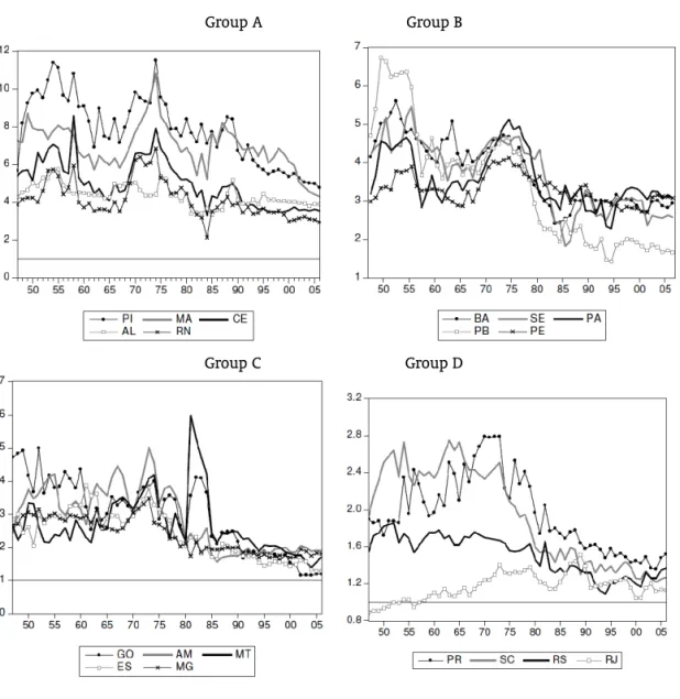
Last, Figure 1 presents the evolution of the ratios between SP and each State income. Using the average income we rank the states, beginning with the poorest ones, to form 4 groups. Thus, Group A is formed by the poorest states (PI, MA, CE, AL and RN) and Group D by the richest ones (SC, RS, RJ and PR). Once again, values greater than 1 (horizontal line) mean that SP is richer than the compared state. In general, the ratios become closer to one, approaching SP. However, this visual inspection is not enough to find convergence. We need to move forward, testing formally this possibility. Indeed, if for the whole period most states approach SP, on the other hand, at least for some of them from 1995 to 2006 the ratio is very flat.
4. RESULTS
To have a benchmark of the cross-section approach, we estimated the usual regression to test un-conditional convergence:
lnYi,T −lnYi,0=a+blnYt,0+εi,T
where Yi,T is the income level of State i at periodτ. This regression represents the core of
Graph 2 – Box plot of the ratio between SP and other states (poorest)
Looking at the initial level of income, there are also two remarkable states, SP (18.51) and RJ (20.90). We run the regression again by means of the LAD estimator, which is robust to outliers, and the coefficient
bbecomes insignificant at 5% level.16
In 2006 the Brazilian GDP growth rate was very large relative to 2001, for instance. Thus, to check the robustness of the result we also analyzed the period from 1947 to 2001, using a recession year to calculate the growth rate. The results are qualitatively the same. The OLS found a coefficient around
−0.03which is significant at 5% level (see Graph 4). However, once again the coefficient implies a very low converge rate. Indeed, the LAD estimator obtained an insignificant coefficient.
Although these analyses should be viewed with caution, given the low number of cross-section units and the absence of conditioning variables, at least we can safely say that (unconditional) convergence is not an obvious result.
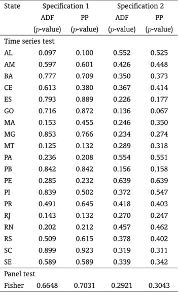
Now we turn to time series approach, beginning our analysis with the unit root tests. We applied the augmented Dickey-Fuller (ADF) and Phillips-Perron (PP). Two specifications were considered, the first contains a constant, while the second does not have any deterministic component. If the unit root null hypothesis is rejected in specification 1, it does not mean that the states are convergent, once in the long-run they deviate by a constant. The specification 2 does not have a constant, constituting a proper test of convergence. The results are displayed in Table 1. Using the 5% level of significance, the ADF and PP tests do not reject the null hypothesis for any state and specification. At 10% level of significance, the ADF test is able to reject the null hypothesis only for AL in specification 1, while the PP test rejects the unit root only for GO in specification 2. Therefore, there is strong evidence against convergence, even when we allow the states to deviate from SP by a constant term. Given the result of the cross-section
Figure 1: Income ratio evolution
Group A Group B
Graph 3 – Unconditional beta convergence analysis, 1947-2006
approach, even if the convergence took place in this period, the convergence rate would be very low, precluding the unit root tests to reject a false unit root null hypothesis.
In an attempt to increase the power of the unit root tests, Maddala e Wu (1999) used Fisher’s (1932) results to derive a test that combine thep-values from individual tests, obtaining a panel test. Define
πias thep-value from any individual unit root test for cross-sectioni,1, . . . ,N. Then, under the null
hypothesis of unit root for allNcross-sections, the following asymptotic result is valid
−2 N X
i=1
log(πi)→χ22N
Graph 4 – Unconditional beta convergence analysis, 1947-2001
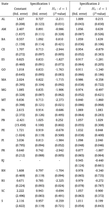
Finally, we employ the ARFIMA models to estimate the decay rated. Following the strategy of the unit root tests, we consider two specifications. The first contain a constant and the second does not have any deterministic term. The results are displayed in Table 2. First of all, it is worth mentioning that the procedure to estimatedfor RJ did not converge when the specification 1 was employed. Allowing the constant term, in the fashion of Azzoni e Barossi-Filho (2002), 16 states present a point estimated of
din the interval(−1/2,1). For 5 (11) states we are able to reject the null hypothesisd= 1at 5% (10%) level. Thus, as the constant term is frequently significant, it seems that most states deviate from SP by a constant value. Looking at the results of specification 2, the number of states with point estimate of
dlower than 1, reduced to 10. From this subgroup only MT and PR rejected the null hypothesisd= 1, still for a 10% significance level. Then, so far, there is a lack of convergence across Brazilian States.
To check the robustness of the results we apply the QMLE estimator. To implement this method, it is necessary to choose the value of the bandwidthm. Robinson (1995a) proposed thatmshould be smaller than T/2 to avoid aliasing effects. Indeed, while some authors have adopted T/2 as the upper bound to the grid of m, others lie in the interval[T1/2
,T4/5
].17 The first option implies a value ofm less than or equal to 30, while the second approach implies a range from 7 to 27. Thus, we estimated the model allowingmto vary from 7 to 30. Since the time series are clearly nonstationary, the analysis
Table 1: Results of unit root tests – Sample: 1947-2006
State Specification 1 Specification 2
ADF PP ADF PP
(p-value) (p-value) (p-value) (p-value) Time series test
AL 0.097 0.100 0.552 0.525
AM 0.597 0.601 0.426 0.448
BA 0.777 0.709 0.350 0.373
CE 0.613 0.380 0.367 0.414
ES 0.793 0.889 0.226 0.177
GO 0.716 0.872 0.136 0.067
MA 0.153 0.455 0.246 0.350
MG 0.853 0.766 0.234 0.274
MT 0.125 0.132 0.289 0.318
PA 0.236 0.208 0.554 0.551
PB 0.842 0.842 0.156 0.158
PE 0.285 0.232 0.639 0.639
PI 0.839 0.502 0.372 0.547
PR 0.491 0.645 0.418 0.403
RJ 0.143 0.132 0.270 0.247
RN 0.202 0.212 0.457 0.462
RS 0.509 0.615 0.378 0.402
SC 0.899 0.923 0.319 0.311
SE 0.589 0.589 0.339 0.342
Panel test
Fisher 0.6648 0.7031 0.2921 0.3043
Table 2: Results of ARFIMA(0,d,0)model – Sample: 1947-2006
State Specification 1 Specification 2 Constant d H0:d= 1 d H0:d= 1
(Std. error) (Std. error) (P-value) (Std. error) (P-value)
AL 1.627 0.727 -2.211 1.009 0.215
(0.208) (0.123) (0.031) (0.043) (0.830)
AM 2.407 0.891 -0.986 1.056 0.639
(1.837) (0.111) (0.328) (0.087) (0.526)
BA 0.557 1.092 0.810 1.059 1.639
(1.159) (0.114) (0.421) (0.036) (0.106)
CE 1.707 0.713 -2.944 0.954 -0.879
(0.272) (0.097) (0.005) (0.052) (0.383)
ES 0.825 0.833 -1.827 0.917 -1.281
(0.460) (0.091) (0.073) (0.064) (0.205)
GO 1.018 0.833 -1.763 0.911 -1.340
(0.645) (0.095) (0.083) (0.066) (0.186)
MA 2.024 0.822 -1.715 0.986 -0.358
(0.395) (0.104) (0.092) (0.038) (0.722)
MG 1.085 0.835 -1.906 0.974 -0.497
(0.328) (0.087) (0.062) (0.052) (0.621)
MT 0.836 0.713 -2.373 0.840 -1.860
(0.398) (0.121) (0.021) (0.086) (0.068)
PA 2.615 0.914 -0.686 1.069 1.083
(2.372) (0.126) (0.495) (0.064) (0.283)
PB -2.421 1.025 0.252 1.057 1.029
(15.450) 0.100) (0.802) (0.055) (0.308)
PE 1.721 0.919 -0.678 1.032 0.848
(1.024) (0.119) (0.500) (0.038) (0.400)
PI 3.036 0.813 -1.984 1.098 2.040
(0.795) (0.094) (0.052) (0.048) (0.046)
PR 0.640 0.742 -2.942 0.877 -1.887
(0.212) (0.088) (0.005) (0.065) (0.064)
RJ - - - 0.945 -0.440
(0.124) (0.661)
RN 1.608 0.797 -1.704 0.978 -0.340
(0.469) (0.119) (0.094) (0.065) (0.735)
RS 0.671 0.785 -2.325 0.979 -0.272
(0.224) (0.093) (0.024) (0.078) (0.787)
SC 2.222 0.943 -0.694 1.057 0.900
(2.496) (0.083) (0.491) (0.063) (0.372)
S 2.116 0.957 -0.359 1.011 0.199
(2.822) (0.119) (0.721) (0.054) (0.843)
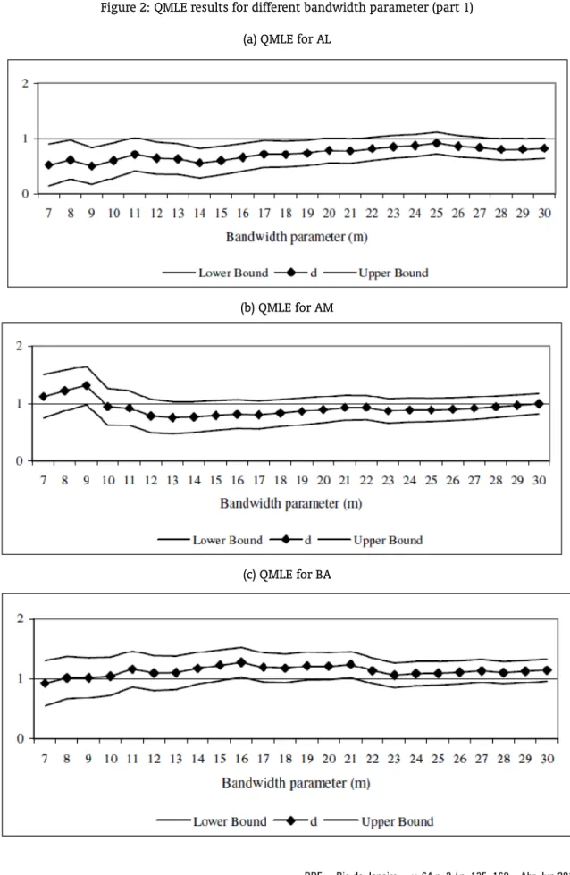
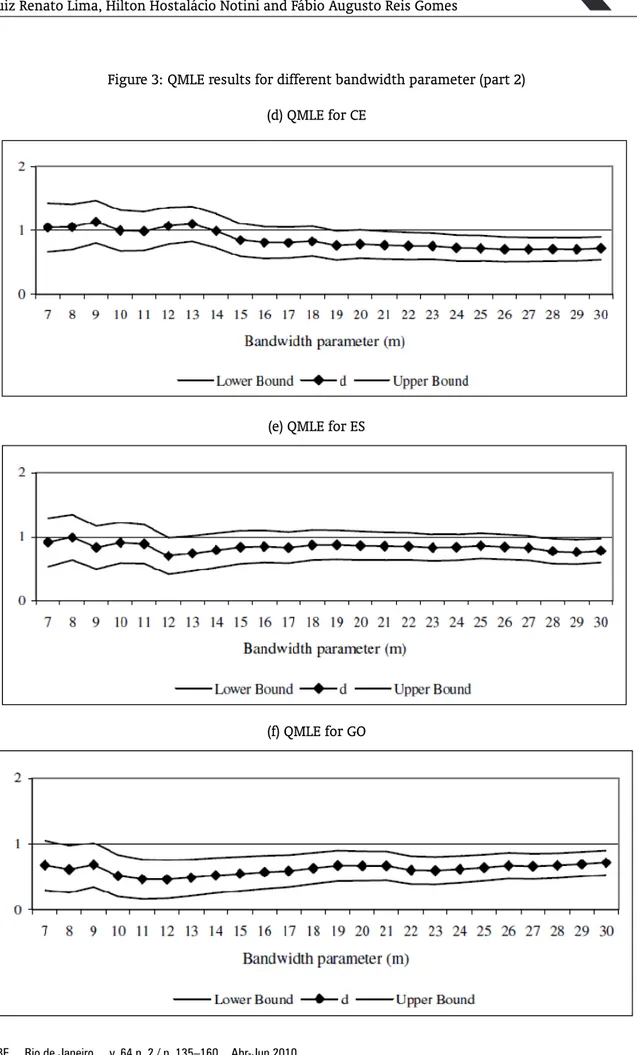
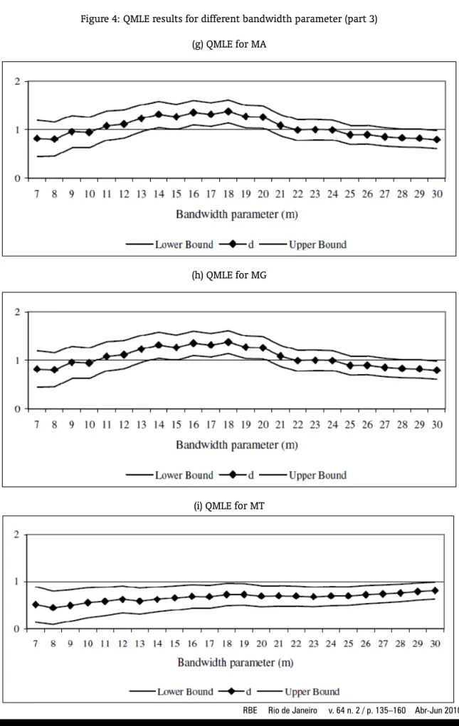
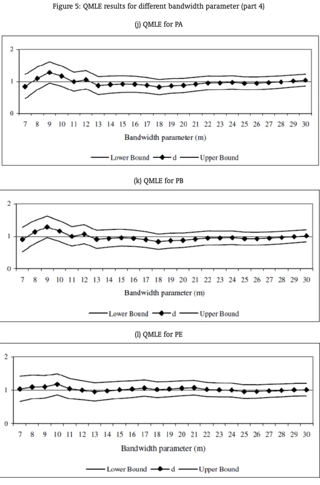
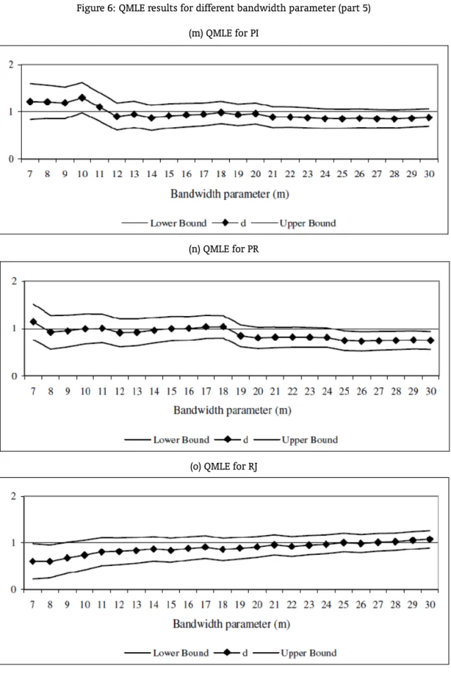
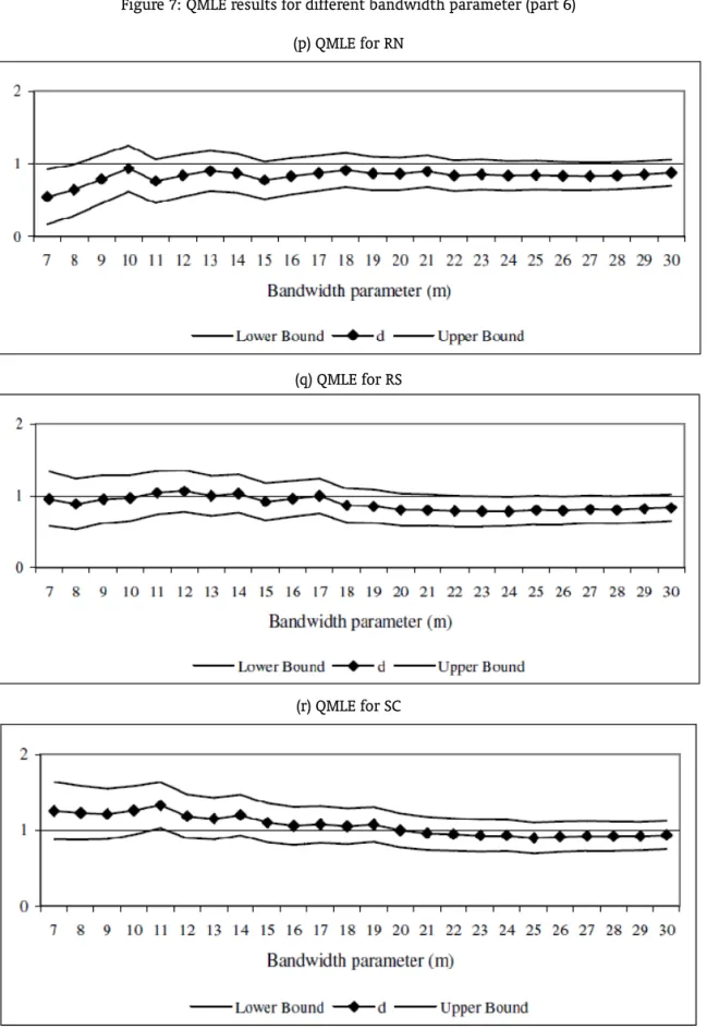
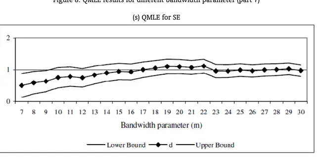
will be carried out based on the first differenced data. To obtain the proper orders of integration of the series we just need to add 1 to the coefficient of the first differenced series. Figure 2 displays the results. In the graphs, the vertical axis refers to the order of integration, while the horizontal one corresponds to the bandwidth parameter numberm. Thus, for each State, the Graph shows the value ofdand its confidence interval for each value ofm.18
Seven states – AM, BA, PA, PB, PE, PI and SC – present a confidence interval which contains the unitary value for all values ofm. Thus, we can safely say that there is no evidence of convergence for these states. The confidence interval of eight states – ES, MA, MG, PR, RJ, RN, RS and SE – contains the unitary value for most values ofm. Hence, the main clonclusion would be against convergence. CE did not reject the unitary value for approximately 50% of the cases while AL did not reject for 37%. In these cases, there is no a clear evidence against or in favor of convergence. GO did not reject the unitary value two times while the confidence interval of MT is always below one. Therefore, there is a strong sign of convergence for GO and MT.
Summarizing, the PP unit root test showed evidence of convergence only for GO; the NLS method to estimate the ARFIMA model presented signs of convergence only for MT and PR, while the QMLE found reliable evidence of convergence for GO and MT. After all, the findings can cast doubts on the convergence hypothesis for the country as a whole. The evidence of convergence toward SP is more robust only for GO and MT.
5. CONCLUSION
In this paper we test the real convergence hypothesis across Brazilian States using unit root tests and ARFIMA models. In particular, we have examined the order of integration of the annual log real per capita Gross State Product (GSP) series for twenty states, taking SP as a benchmark. In general, our results suggest a lack of convergence. It is worth mentioning that the time series approach does not include any covariate and, as a consequence, it can be viewed as an unconditional test.
It is important to say that our time series results are very different from the works of Ferreira e Diniz (1995), Schwartsman (1996), Ellery Jr. e Ferreira (1996) and Ferreira (2000) which used a cross-sectional approach to study convergence across Brazilian States. While these studies show that the states are convergent, we found the opposite result. One possible explanation is the broader time period used in here than the cross-section studies (which usually cover the period 1970-1995). Besides, it is relevant to stress that our analysis brings much more information about income convergence as we test the convergence hypothesis for each state separately. In a cross-sectional approach, instead, it is not possible to conclude which state is converging to the benchmark state and which is not.
Our results are not directly compared with the ones from Azzoni e Barossi-Filho (2002) because the two works used different benchmarks. While we adopted São Paulo as our benchmark for the convergence analysis, Azzoni e Barossi-Filho (2002) chose the nation per capita income. It is important to mention that the employment of long memory models and unit root tests with structural breaks share the same purpose: improve the power to reject a false unit root. However, as mentioned the unit root tests with endogenously structural break points are very sensitive to the specification of the alternative model (Montañés et alii, 2005), and the model does not impose that the income differences will have a mean zero in the long-run. Despite all differences, our results are not incompatible with those from Azzoni e Barossi-Filho (2002). While our finding casts doubts on convergence toward SP, they found a convergent group that does not include SP.
Last, as discussed by Campbell e Perron (1991), long time series are more susceptible to presence of structural breaks. As discussed by Perron (1989, 1997), the omission of structural breaks leads the ADF test to not reject a false unit root hypothesis. In addition, Diebold e Inoue (2001) wrote that the long-memory literature has not paid enough attention to the possibility of confusing structural
Figure 2: QMLE results for different bandwidth parameter (part 1)
(a) QMLE for AL
(b) QMLE for AM
Figure 3: QMLE results for different bandwidth parameter (part 2)
(d) QMLE for CE
(e) QMLE for ES
Figure 4: QMLE results for different bandwidth parameter (part 3)
(g) QMLE for MA
(h) QMLE for MG
Figure 5: QMLE results for different bandwidth parameter (part 4)
(j) QMLE for PA
(k) QMLE for PB
Figure 6: QMLE results for different bandwidth parameter (part 5)
(m) QMLE for PI
(n) QMLE for PR
Figure 7: QMLE results for different bandwidth parameter (part 6)
(p) QMLE for RN
(q) QMLE for RS
Figure 8: QMLE results for different bandwidth parameter (part 7)
(s) QMLE for SE
breaks and long memory processes. Indeed, Granger e Hyung (2004) showed that omitting occasional breaks lead to an overestimatedd. Therefore, the omission of structural breaks will overestimate the evidence against convergence. However, this analysis is beyond the scope of this paper because the introduction of determinist term implies that income difference will not converge to zero. The inclusion of determinist term,d(t), demand a new approach where thed(t)vanishes astgoes to infinity.
BIBLIOGRAPHY
Attfield, C. L. F. (2003). Structural breaks and convergence in output growth in EU. Department of Economics, University of Bristol, Discussion Paper 03/544.
Azzoni, C. (1997). Concentração regional e dispersão das rendas per capita estaduais: Análise a partir de séries históricas estaduais de PIB (1939-1995). Estudos Econômicos, 27:341–393.
Azzoni, C. & Barossi-Filho, M. (2002). A time series analysis of regional income convergence in Brazil. In Anais do XXX Encontro Nacional de Economia, Nova Friburgo. ANPEC.
Azzoni, C., Menezes-Filho, N., Menezes, T., & Silveira-Neto, R. (2000). Geography and regional income inequality in Brazil. Inter American Development Bank, Working Paper.
Baillie, R. T. (1996). Long memory processes and fractional integration in econometrics. Journal of Econometrics, 73:5–59.
Barro, R. (1991). Economic growth in a cross-section of countries. Quarterly Journal of Economics, CVI:407–55.
Barro, R. & Sala-i-Martin, X. (1992). Convergence.Journal of Political Economy, 100:223–51.
Bernard, A. B. & Durlauf, S. N. (1991). Convergence of international output movements. NBER Working Papers 3717, National Bureau of Economic Research, Inc.
Bernard, A. B. & Durlauf, S. N. (1996). Interpreting tests of the convergence hypothesis. Journal of Econometrics, 71:161–173.
Campbell, J. Y. & Mankiw, N. G. (1989). International evidence on the persistence of economic fluctua-tions.Journal of Monetary Economics, 23:319–333.
Campbell, J. Y. & Perron, P. (1991). Pitfalls and opportunities: What macroeconomists should know about unit roots. InMacroeconomic Annual, pages 141–201. NBER.
Carlino, G. A. & Mills, L. O. (1993). Are U.S. regional incomes converging? A time series analysis.Journal of Monetary Economics, 32:335–346.
Carvalho, F. & Santos, C. (2007). Dinâmica das disparidades regionais da renda per capita nos estados brasileiros: Uma análise de convergência. Revista Economia e Desenvolvimento, 19:78–91.
Diebold, F. X. & Inoue, A. (2001). Long memory and regime switching.Journal of Econometrics, 105:131– 159.
Diebold, F. X. & Rudebusch, G. D. (1991). On the power of Dickey-Fuller tests against freactional alterna-tives.Economics Letters, 35:155–160.
Durlauf, S. N. (2001). Manifesto for a growth econometrics. Journal of Econometrics, 100:65–69.
Durlauf, S. N. & Johnson, P. A. (1995). Multiple regimes and cross-country growth behaviour. Journal of Applied Econometrics, 10:365–84.
Ellery Jr., R. & Ferreira, P. C. (1996). Crescimento econômico e convergência entre a renda dos estados brasileiros.Revista de Econometria, 16:83–104.
Ferreira, A. H. B. (1999). Concentração regional e dispersão das rendas per capita estaduais: Um comen-tário. Estudos Econômicos, 29:47–63.
Ferreira, A. H. B. (2000). Convergence in Brazil: Recent trends and long run prospects.Applied Economics, 32:479–489.
Ferreira, A. H. B. & Diniz, C. C. (1995). Convergência entre as rendas per capita estaduais no Brasil. Revista de Economia Política, 15:38–56.
Fisher, R. (1932).Statistical Methods for Research Workers. Oliver & Boyd, Edinburgh.
Geweke, P. & Porter-Hudak, S. (1983). The estimation and application of long memory time series models. Journal of Time Series Analysis, 4:221–38.
Gil-Alana, L. A. (2002). Comparisons between semiparametric procedures for estimating the fractional differencing parameter. Preprint.
Gil-Alana, L. A. (2003). Long memory in financial time series with non Gaussian disturbances. Interna-tional Journal of Theoretical and Applied Finance, 6:119–134.
Gonzalo, J. & Lee, T.-H. (2000). On the robusteness of cointegration tests when series are fractionally integrated. Open access publications from Universidad Carlos III de Madrid info:hdl:10016/3565, Universidad Carlos III de Madrid.
Granger, C. & Joyeux, R. (1980). An introduction to long memory time series models and fractional differencing. Journal of Time Series Analysis, 1:15–39.
Granger, C. W. J. & Hyung, N. (2004). Occasional structural breaks and long memory with an application to the S&P 500 absolute stock returns. Journal of Empirical Finance, 11:399–421.
Hassler, U. & Wolters, J. (1994). On the power of unit root tests against fractional alternatives.Economics Letters, 45:1–5.
Johansen, S. (1988). Statistical analysis of cointegration vectors. Journal of Economic Dynamics and Control, 12:231–54.
Kramer, W. (1998). Fractional integration and the augmented Dickey-Fuller test. Economics Letters, 61:269–272.
Kunsch, H. (1986). Discrimination between monotonic trends and long range dependence. Journal of Applied Probability, 23:1025–30.
Li, Q. & Papell, D. H. (1999). Convergence of international output: Time series evidence for 16 OECD countries. International Review of Economics and Finance, 8:267–280.
Maddala, G. & Wu, S. (2000). Cross-country growth regressions: Problems of heterogeneity, stability and interpretation.Applied Economics, 32:635–642.
Maddala, G. S. & Wu, S. (1999). A comparative study of unit root tests with panel data and new simple test. Oxford Bulletin of Economics and Statistics, 61:631–652.
Mankiw, G., Romer, P., & Weil, D. N. (1992). A contribution to the empirics of economic growth.Quarterly Journal of Economics, 107:407–37.
Mello, M. & Guimarães-Filho, R. (2007). A note on fractional stochastic convergence. Economics Bulletin, 3:1–14.
Menezes, T. & Azzoni, C. (2000). Convergência de renda real e nominal entre regiões metropolitanas brasileiras: Uma análise de dados de painel. In Anais do XXVIII Encontro de Economia, Campinas. ANPEC.
Michelacci, C. & Zaffaroni, P. (2000). Fractional beta convergence.Journal of Monetary Economics, 45:129– 153.
Montañés, A., Olloqui, I., & Calvo, E. (2005). Selection of the break in the Perron-type tests. Journal of Econometrics, 129:41–64.
Perron, P. (1989). The great crash, the oil price shock and the unit root hypothesis. Econometrica, 57:1361–401.
Perron, P. (1997). Further evidence on breaking trend functions in macroeconomic variables. Journal of Econometrics, 80:355–385.
Quah, D. (1995). Empirics for economic growth and convergence. European Economic Review, 40:1353– 75.
Robinson, P. M. (1995a). Gaussian semiparametric estimation of long range dependence. Annals of Statistics, 23:1630–61.
Robinson, P. M. (1995b). Log-periodogram regression of time series with range dependence. Annals of Statistics, 23:1048–72.
Sala-i-Martin, X. (1996). The classical approach to convergence analysis.The Economic Journal, 106:1019– 1036.
Schwartsman, A. (1996). Convergence across Brazilian states. Discussion Paper 02/96. IPE, Universidade de São Paulo.