Sergio Guimar˜aes Ferreira**
Summary: 1. Introduction; 2. Theoretical framework; 3. The college wage premium and the relative supplies of college workers by age; 4. The effect of cohort-specific supplies on the college wage premium of male workers; 5. Screening the college-high school ratio between age and cohort effects; 6. Conclusion.
Keywords: college premium; pseudo panel; labor supply; elasticity of substitution.
JEL codes: J31; C23.
Esse artigo testa a existˆencia de rela¸c˜ao causal entre a evolu¸c˜ao da oferta de trabalhadores com qualifica¸c˜ao universit´aria e a perfor-mance do diferencial salarial entre trabalhadores com n´ıvel univer-sit´ario e trabalhadores com n´ıvel secund´ario, no Brasil. Gradua¸c˜ao tardia causa problema de composi¸c˜ao amostral que potencialmente viesa o impacto da oferta de trabalho sobre o premio salarial. Eu estimo o impacto da oferta relativa no diferencial de salarios, com e sem controlar os efeitos da gradua¸c˜ao tardia. Em ambos os casos, eu encontro coeficientes de elasticidade de substitui¸c˜ao baixo entre trabalhadores qualificados e n˜ao qualificados. Contudo, o procedi-mento adotado afeta decisivamente conclus˜oes sobre a elasticidade de substitui¸c˜ao entre diferentes grupos et´arios.
This paper tests the existence of causal relationship between the evolution of college-educated labor supply and the performance of the college premium in Brazil. Late college graduation causes sam-pling composition problem which may bias the impact of labor sup-ply on the college premium. I estimate the impact of the relative supply of college-educated labor on wage, with and without con-trolling for the composition bias. In both cases, I find a relatively low elasticity of substitution between school groups. However, the estimate of the partial elasticity of substitution between age groups is crucially affected by the chosen estimation procedure.
*
This paper was received in Apr. 2003 and approved in Feb. 2004. I thank the valuable comments of John Karl Scholz, Rodolfo Manuelli, Cristina Terra, Hugo Boff, Francisco Ferreira, Gustavo Gonzaga, Naercio Menezes, Reynaldo Fernandes, as well as other participants of seminars at the University of Wisconsin – Madison, FGV-RJ, IBMEC-SP, USP, LACEA and IPEA. The usual disclaims also apply.
**
1.
Introduction
Education attainment of the labor force has mildly increased in the last two decades in Brazil. I am interested in testing if the increase in the number of workers with a college degree has somewhat led to a downward pressure in the college wage premium. The premium is defined as the wage difference between workers with a college degree and workers with a high school degree.
There is recent work that examines the effects of supply changes on the returns to education in the US, Canada and UK. The seminal work, by Katz and Murphy (1992) looks at movements in the college wage premium in the US from 1963 to 1987 and concludes that “it appears to be strongly related to fluctuations in the rate of growth of the supply of college graduates”. Their model assumes perfect substitutability among workers in different age groups as long as they have the same level of education. Such an assumption allows them to construct an aggregate education index as a linear combination between the “amount of education” supplied by workers of different ages.
Card and Lemieux (2001) extend Katz and Murphy’s model to allow imper-fect substitution between workers of different ages. By measuring the impact of changes in the supply of education (of different age groups) on the college wage premium, they are able to estimate the elasticity of substitution between different age groups with the same education level. Once they estimate this parameter, they are able to calculate aggregate indexes for the total supply of high school and college workers in the labor force that take into account the imperfect substitution among age groups. Their estimates for the US suggest that the elasticity of sub-stitution between different age groups is large but finite at 4.4, while the elasticity of substitution between college and high school labor types is in the range of 1.1 to 1.6. Results are similar for both the UK and Canada.
college labor in period t, and on the age-group specific relative supply of college labor.
The econometric method consists on constructing a pseudo panel of cohort groups. In the first step, I estimate the partial elasticity of substitution among age groups within each educational category in order to calculate aggregates for the two labor types. The second step consists on the estimation of the elasticity of substitution between the two labor types, college and high school types.
One important issue is how to correctly identify changes in demand for skills from changes in the supply of skills. Card and Lemieux (2001) and Katz and Mur-phy (1992), among others, assume that the effect of skill-biased technical change on college wage premium can be summarized by a time trend. This assumption may be questionable for the Brazilian economy, since some authors argue in favor of the presence of a structural break on the impact of demand on the relative price of skills, in the 1990s (e.g. Fernandes and Menezes (2001)).1 I allow for this possibility by adding cohort dummies which can partly capture non linear varia-tions over time in the relative demand for skills. In this paper, I get very small (statistically not significant) impact of age-specific supply on age-specific school premium when not controlling for life cycle variations in school supply. Due to a substantial presence of late graduation in the Brazilian data, there is a clear positive relationship between age and relative supply of college-type labor. Life cycle changes in the supply of schooling are shown to be positively correlated to life cycle changes in wage differentials.
Once I decompose changes in the supply of schooling between life cycle and cohort components, I find that cohort-specific relative supply is negatively corre-lated to schooling premium: a 10% increase in college-educated supply for a given age group will lead to a 2.2% fall on college premium for that particular age group. The paper has six additional sections. In section 2, the theoretical model is presented. Section 3 presents the empirical procedure. Section 4 presents the selected sample, and explains how I constructed the panel of wage gaps and school-related labor indexes. In addition, it presents how the constructed series have evolved over time. Section 5 presents the result of the estimations, when I do not control for the effects of late graduation in the supply of college-type workers. In section 6, I treat the data for potential presence of life cycle bias and estimate again the partial elasticity of substitution. Section 7 concludes the paper.
1
2.
Theoretical Framework
Aggregate output depends on two CES sub-aggregates of high school and col-lege labor:
Ct= [
X
j
(αjtCjtη)]1/η (1)
and
Ht= [
X
j
(βjtHjtη)]1/η (2)
where −∞ < η ≤ 1 is a function of the partial elasticity of substitution σA
between different age groups j with the same level of education (η = 1−1/σA).
Each age group has specific relative efficiency parameters,αjt andβjt, which vary
over time. In other words, those parameters may suffer influence of cohort-specific productivity shocks (e. g. variation in school quality).2
In the limiting case of perfect substitutability across age groups,ηis equal to 1 and total high-school (or college) labor input is a weighted sum of the quantity of labor supplied by each age group. I assume that the aggregate production function is also CES:
yt= (θctCtρ+θhtHtρ)1/ρ (3)
where −∞< ρ ≤1 is a function of the elasticity of substitution σE between the
two education groups (ρ= 1−1/σE). In this setting, the marginal product of labor
for a given age-education group depends on both the group’s own supply of labor and the aggregate supply of labor in its education category. Efficient utilization of different skill groups requires that relative wages are equated to relative marginal products:3
ln(wjtH) = ln(∂yt/∂Hjt) = ln(θhtHtρ−ηΨt) + ln(βjt)−1/σAlnHjt (4)
ln(wjtC) = ln(∂yt/∂Cjt) = ln(θctCtρ−ηΨt) + ln(αjt)−1/σAlnCjt (5)
2
In addition, suchαjt andβjt may capture structural breaks in the demand for skills
poten-tially driven, for example, by trade liberalization.
3
∂yt/∂Hjt =∂yt/∂Ht∂Ht/∂Hjt =θhtHρ− 1
t ΨtβjtHη− 1 jt H
1−η
t = θhtHtρ−ηΨtβjtHη− 1 jt .
ψt= (θctCtρ+θhtHtρ)1/ρ−1 (6)
Equations (4) and (5) imply that the ratio of the wage rate of college workers in age group j(wjtc) to the wage of high-school workers in the same age group
j(wH
jt) satisfies to the following equation:
ln(wCjt/wHjt) = ln(θCt/θHt) + ln(αjt/βjt) + (1/σA (7)
− 1/σE) ln(Ct/Ht)−1/σAln(Cjt/Hjt)
Hence, if the relative employment ratios are exogenous, equation (7) leads to a model for the observed college-high school wage gap rjt of workers in age group
j in year t:
rjt ≡ ln(wCjt/wHjt) = ln(θCt/θHt) + ln(αjt/βjt)
+ (1/σA−1/σE) ln(Ct/Ht)−(1/σA) ln(Cjt/Hjt) +ejt (8a)
whereejtreflects sampling variation in the measured gap and/or any other sources
of variations in age-specific wage premiums.4
According to equation (8a), the college-high school gap for a given age group depends on both the aggregate relative supply of college labor (Ct/Ht) in period
t, and on the age-group specific relative supply of college labor (Cjt/Hjt). When
there is perfect substitution across age groups with the same level of education, the college premium will depend only on the aggregate relative supply of college workers, on the relative technology shock θct/θht, and on the age-cohort relative
efficiency parameter βjt/αjt.
For purposes of estimation, it is convenient to rearrange equation (8a) in an alternative form:
rjt = ln(θCt/θHt) + ln(αjt/βjt)−(1/σE) ln(Ct/Ht)−(1/σA)[ln(Cjt/Hjt)
− ln(Ct/Ht)] +ejt (8b)
4
3.
Econometric Method
The primary purpose of this paper is to estimate the effect of the aggregate relative supply of college labor on the college-high school wage gap. A problem arises in the attempt to estimate Equation (8a) because aggregate supplies of the two types of labor (Ct and Ht) depend on the elasticity of substitution across
age groups, according to equations (1) and (2). Following Card and Lemieux (2001), a two-step estimation provides a method for identifying both σA and σE.
In the first step, σA is estimated from a regression of age-group specific college
wage gaps on age group-specific relative supplies of college educated labor, cohort effects (which absorb the relative productivity effect, ln(βjt/αjt)), and time effects
(which absorb the combined relative technology shock and any effect of aggregate relative supply):
rjt =bt−j +dt−(1/σA) ln(Cjt/Hjt) +ejt (9)
where bt−j are cohort dummies and dt are time dummies. Given an estimate of
1/σA, the relative efficiency parametersαjt andβjt are easily computed by noting
that equations (4) and (5) can be transformed into:
ln(wjtH) + 1/σAlnHjt= ln(θhtHtρ−ηΨt) + ln(βjt) (10)
ln(wjtC) + 1/σAlnCjt = ln(θctCtρ−ηΨt) + ln(αjt) for allj and t (11)
The left hand side of these equations can be computed directly using the first step estimate of 1/σA. The right hand side can be estimated by a set of time
dummies (first term) and cohort dummies (relative efficiency parameters). Given estimates ofαjt’s,βjt’s and ofη, it is easy to construct estimates of the aggregate
supply of college and high school labor in each year (Ct andHt).
With these estimates in hand, and some assumptions about the time series path of the relative productivity term, log(θct/θht), equation (8b) can be estimated
directly. I follow the previous mentioned literature and assume that log(θct/θht)
can be represented as a linear trend.
4.
The College Wage Premium and the Relative Supplies of
College Workers by Age
supplies of college-educated workers by age group. The data are drawn from the Brazilian Nationwide Household Sample (PNAD), for the years 1976 to 1998.5
The Evolution of the College Wage Premium for Male Workers
6Figure 1 shows the evolution of the overall college premium for male workers since 1977. This premium is measured by the coefficient on a regression of log wage on a college dummy and several control variables, for every year in the sample.7 My estimates of the college wage premiums are based on the total labor earnings (income from all jobs) of men aged 24 to 58, living in urban areas of Brazil, who are either employed or self – employers and are working at least 40 hours in the week of reference. In addition, extremely low and extremely high hourly wage rates are dropped from the sample.8 The remaining sample size is 217,206 observations.The college wage gap has been widening, but not at a constant rate over time. After increasing substantially during the 1980’s and reaching 0.82 in 1990, the
college-5
Data is not available for the following years: 1980, 1991 and 1994.
6
I focus exclusively on the evolution of the college wage gap for men. I believe that this focus is appropriate, given inter-cohort changes in female labor supply that have presumably affected the age profiles of earnings for women in different education groups over the past twenty years. If women in younger cohorts accumulate more actual experience per year of potential experience than older cohorts, this will increase the measured college-high school wage even if the true college premium is fixed. Secular changes in the age profile of the college-high school wage gap may, therefore, be contaminated by these composition effects. Another reason for excluding women from the calculation of the college wage gap is that the sample female hourly labor earnings are very imprecise due to substantial variations in the number of hours worked.
7
The control variables are: a second degree polynomial for age, five regional dummies and a dummy for self employment. Table A.1 shows the cohorts classified by birth year. Table A2 in the Appendix shows the results of the regression for each year.
8
high school differences of the log hourly wage has been oscillating around 0.78 during the 1990’s.9 The college premium increased by 15% from 1977 to 1998, but only 1.2% from 1990 to 1998.
Figure 1
College wage premium (in ln base)
Table 1 presents my estimates of the “college wage premiums” for 5-year age groups, taken at 5-year intervals over my sample period. The estimates are based on differences in mean log average hourly wages between full time workers with a complete or an incomplete college degree (i. e., at least 12 years in school) and those with a complete or an incomplete high school degree (i. e., at least 9 and at most 11 years in school).10 The wage gaps are estimated in separate regression models for each cohort in each “year”.11 Each model includes a dummy for college degree (defined as above), and the following control variables: a linear age term, an indicator of self-employment, five regional dummies, and time dummies.12
Comparisons down a column of the table show the changing college premium for a specific age group. Older workers observe a substantial increase in the college premium over time, especially until 1990. On the contrary, the wage gap is almost the same for younger workers in 1977 and in 1998. One can say that the increase in school premium during the 1980s was pushed by senior workers (more than 34 years old).
9
In 1998, a worker in the college group earned on average 2.3 times more than a worker in the high school group.
10
I can only identify a complete high school or college degree for years after 1992. It is possible that some of the changes in wage can be a result of composition within the education categories, but I do not have how to control for it.
11
The “year” is a pool of three subsequent years. The only exception is the “year” 1991-93, because there was no survey in 1991.
12
Table 1
College – high school wage differentials - only males
year/age 24–28 29–33 34–38 39–43 44–48 49–53 54–58 1976–78 0.714 0.790 0.706 0.725 0.665 0.608 0.772 (.016) (.018) (.023) (.026) (.031) (.041) (.058) 1981–83 0.620 0.725 0.740 0.743 0.703 0.758 0.664 (.015) (.015) (.018) (.024) (.029) (.037) (.052) 1986–88 0.677 0.783 0.822 0.834 0.740 0.857 0.767 (.02) (.019) (.022) (.027) (.037) (.05) (.073) 1991–93 0.657 0.691 0.722 0.791 0.796 0.832 0.874 (.023) (.024) (.026) (.031) (.040) (.058) (.083) 1996–98 0.648 0.767 0.817 0.824 0.808 0.924 0.936 (.018) (.018) (.018) (.021) (.026) (.035) (.054) 1) College dummy coefficients in a regression model that include as control variables. (2) The sample contains a rolling age group. For example, the 24-28 year old group in the 1976-78 sample includes individuals 23-27 in 1976, 24-28 in 1977 and 25-29 in 1978. (3) College workers are defined as workers who got at least incomplete college degree; High School workers are those who are either high school dropouts or high school graduates (exactly 11 years in school). (4) Standard Errors in parentheses
Relative Supplies of College-educated Labor
I turn next to an overview of my estimates of the relative supplies of college-educated labor by age group and year. I estimate relative supplies from a broad sample that includes men and women. My estimates of relative supplies of different education groups are based on data for men and women aged 24 to 58, who had worked as an employee or were self-employer at least one hour in the week of reference. The sample size is 1,803,168 observations. To account for differences in the effective supply of labor by different groups, I count the number of hours worked in the week by each worker and weight these hours by the average wage (over all periods) of his (or her) education group.
Figure 2 shows that there is a clear positive trend on the proportion of workers with more than eleven years in school in the labor force, although this proportion is no bigger than 17% at the end of the sample period.
I define the amount of “high school labor” of age group j in year t (Hjt) as
the total weekly hours13 worked by high school graduates or dropouts in that age range, plus the total hours of elementary school graduates or dropouts (weighted by their wage relative to the high school group).14 The amount of “college labor”
13
I attribute 20 hours worked for individuals who worked less than 40 hours and 40 hours for those working at least 40 hours.
14
of age groupj(Cjt) is defined as the total number of hours worked by workers with
complete or incomplete college degree.15
Figure 2
Proportion of workers with college
In table 2, the ratio of college labor to high school labor increases for each age group, but the growth is significantly bigger for the older age groups. The college-high school labor ratio hardly changes for individuals in the younger age group, while it almost triples for some of the older age groups (e.g. individuals aged 44 to 48).
school”. Both groups are considered in the aggregate labor supply of “high school” workers, with their respective labor efficiency factors. The relative wage of the workers with complete or incomplete elementary school with respect to the wage of “high school workers” is obtained through a regression (for the whole sample period) of the log hourly real wage on a dummy for “high school workers”, regional dummies, a dummy for self employment and a squared polynomial of age. The labor efficiency factor of the “elementary school” group is 0.52. Card and Lemieux (2001) use only high school graduates or dropouts in their measure of “high school labor type”. In addition, they are able to identify high school dropouts and give respective labor efficiency weights for such group of workers, while I have to consider them with the same weight as those workers who has completed high school.
15
Table 2
School supply – relative college labor supply
24–28 29–33 34–38 39–43 44–48 49–53 54–58 1976–78 0.21 0.23 0.17 0.14 0.13 0.11 0.10 1981–83 0.22 0.27 0.25 0.18 0.15 0.13 0.11 1986–88 0.21 0.29 0.29 0.25 0.20 0.15 0.13 1991–93 0.24 0.28 0.32 0.32 0.28 0.22 0.18 1996–98 0.23 0.29 0.32 0.33 0.33 0.30 0.21 (1) High School Labor Supply == number of workers with incom-plete or comincom-plete high school degree (weighted by # weekly hours) + number of workers with elementary school (weighted by # weekly hours and by the relative wage with respect to high school wage). (2) The average relative wage of the elementary school group (at most 8 years in school) is obtained through a regression of log real wage on age, squared age, regional dummies, and self employ-ment dummy. (3) College Labor Supply == number of workers with incomplete or complete college (weighted by # weekly hours). (4) Relative College Labor Supply == college labor supply: high school labor supply. (5) The number of hours worked is represented by 20 (part time) is the individual worked less than 40 hours and 40 if the individual worked at least 40 hours
The combined evidence of the recent evolution of labor supply and school premium in Brazil shows, first, that the older age groups are both the ones which present the higher growth in college premium and the larger increase in college-type labor supply. Second, it shows that both the aggregate college-educated labor supply and the college premium increases simultaneously. From these facts, one can certainly argue that demand factors are driving the evolution of college premium. However, this does not rules out the influence of the supply side on the premium once we correctly control for the effects of demand shifts.
5.
The Effect of Cohort-Specific Supplies on the College Wage
Premium of Male Workers
16I now turn to the estimation of the effects of the relative supply of college educated workers on the college-high school wage gap. Table 3 presents three estimations of the partial elasticity of substitution.17 In all three cases, the impact of the age-specific relative supply of college-educated workers on the college wage gap is not statistically different from zero. This seems to show that the partial elasticity of substitution across age groups is very high.18 Because specification (3) has the most complete set of controls, I assume 1/σA is−.11 for the purpose
of estimating the cohort-specific efficiency parameters αjt and βjt.19
Based on estimates of 1/σA, αjt and βjt, I get estimates of the aggregate
relative supply index.20 Table 4 presents estimates of the second stage models (based on equation (8b)) that include both age-group specific relative supplies of college labor, and the aggregate relative supply index. The relative technology shock variable (ln(θct/θht) is assumed to follow a linear trend. All the specifications
include cohort and age dummies, as well as a time trend.21
In column (1), I use the estimated aggregate supply of college and high school educated workers as the measure of labor supply. The estimation of equation (8b) shows that the increase in the aggregate supply of college workers substantially
16
For all the estimations in this paper, I assume that men and women are perfectly substi-tutable in the labor force, with identical productivity parameters for a given age and cohort group. This assumption allows me to pool the male and female labor supply and test the impact of it on the college premium of male workers.
17
In column (1), the specification includes time and cohort dummies. In the second specifi-cation, the time dummies are replaced by a linear time trend. In the third specifispecifi-cation, I use a time trend, age dummies and cohort dummies as controls.
18
One has to be careful about the ability to identifying the age, cohort and time coefficients. Since Age = Time – Birth Year, the identification of these effects cannot be done without ad-ditional assumptions. In specification (1), cohort dummies capture both age effects and cohort-specific fixed effects of the wage gap. In cohort-specification (2), the cohort dummies will capture transitory time effects as well (for example, business cycle effects on the college premium), since the time dummies are replaced by a time trend. In specification (3), the life cycle shape of labor earnings is assumed to be fixed over time (captured by the age dummy coefficients), and cohort dummies capture changes in such shape as well as cohort-specific fixed effects and transitory time effects.
19
In the appendix A, table A.3 shows the estimated coefficients for all age and cohort dummies in the stage one.
20
In the appendix A, figure A.1 shows the relative aggregate college-labor supply.
21
depressed the college premium in the last twenty years in Brazil. A 10% increase in the relative supply of college-educated workers drives down the college-high school wage differential by 5.2%, in the absence of non-neutral technology changes. This is compatible to an elasticity of substitution between college and high school workers of 1.93.22
Table 3
Estimated models for the college – high school wage gap, by Cohort and year
(1) (2) (3)
Age group specific 0.06 0.015 -0.111 Relative supply (.129) (.135) (.268)
Trend 0.044 0.033
(.013) (.389) Year effects:
1997 -0.087 (.029) 1982 -0.076 (.024) 1992 -0.007 (.029)
1997 0.079
(.036)
Degrees of freedom 19 22 17
R-squared 0.85 0.79 0.89
OBS: Standard errors in parentheses.Models are estimated by weight least squares.The dependent variable is the college-high school wage gaps shown in table 1. Weights are inverse sampling variances of the estimated wage gaps. All models include cohort effects. Model (3) includes age effects as well. The years indicated when reporting the estimated year effects are the mid-points of the year intervals shown in table 1.
The time trend coefficient is 0.08 and it is significant at 5%. This means that, absent the age/cohort productivity factor and the changes in school supply, the college wage gap would have increased on average by 8% in each 5-year period.23 This might be an effect of skill-biased technology changes, or it may an effect of trade liberalization. Alternatively, this may be an effect of accumulation of
phys-22
Does the estimate of the elasticity of substitution between school groups change if I assume infinite partial elasticity between age groups? In columns (2), I adopt the simple aggregation of college and high school workers across age, assuming perfect substitution across age-groups, as done in Katz and Murphy (1992). In this case, the estimate of the elasticity of substitution between school groups decreases slightly to 1.67.
23
ical capital, if capital is complementary to skilled labor and substitute to unskilled labor.
Table 4
Models for the college-high school wage gap, equation 8b
(1) (2)
Age-specific -0.063 -0.07
Relative supply (.236) (.234)
Trend 0.083 0.094
(.039) (.041) Aggreg. supply index -0.519
for men and women (.287)
Katz-Murphy aggr. supply -0.599
Index (.301)
Degree of freedom 16 16
R-squared 0.92 0.92
OBS: standard errors in parentheses. Models included age and cohort effects.
A 10% increase in the age-specific relative supply of college-educated workers decreases the college premium by only 0.6%, for that particular age-group.24 This implies a very large partial elasticity of substitution of 15.9. Most of the individuals in the sample are low skill workers, performing basic tasks. One might believe that the learning-by-doing content of such jobs are limited, and job-experience should not contribute significantly for labor productivity. In that case, one should expect high substitutability between experienced workers and apprentices.
However, it remains a suspicion that life cycle variations may be creating some noise and biasing the results of OLS regression. Suppose that one believes that age variations inCjt/Hjt are larger for cohorts which faced perspectives of larger
schooling premium. For example, individuals invest in college education once they predict higher schooling premium. Hence cohorts entering in the labor force during an economic boom would show larger than average growth inCjt/Hjt over the life
cycle. In this case, the life cycle component ofCjt/Hjtwould be endogenous while
the cohort component of Cjt/Hjt would be a result of educational policy.25 In
the next section, I filter Cjt/Hjt from the age component in order to get some
cohort-specific schooling supply.
24
Controlling for age dummies changes the coefficient on the aggregate index from -.44 to -.52, but the age-specific supply coefficient goes from -.007 to -.063.
25
6.
Screening the College-High School Ratio between Age and
Co-hort Effects
I can decompose the relative supply of college-educated workers into two com-ponents: an age-specific component ( ˆφj) and a cohort-specific component (λt−j).
This specific decomposition assumes that there is an age profile that is common across different cohorts.26 The log of the relative supply of college-educated work-ers will become:
ln(Cjt/Hjt) =λt−j+φj +ujt (12)
The regression of ln(Cjt/Hjt) in a series of age and cohort dummies in order
to find ˆφj and ˆλt−j shows that all dummies are statistically significant.
27 Once
I calculate ˆλt−j, I can use it to estimate the partial elasticity of substitution
between age groups, instead of using ln(Cjt/Hjt). Table 5 presents the estimation
of equation (9), modified by the presence of ˆλt−j:
rjt =bt−j +dt−(1/σA)λt−j+ejt (13)
This two-stage procedure leads to much stronger effect of age-specific labor supply on age-specific college premium, since it eliminates the downward bias caused by the positive correlation between φj and life cycle changes in schooling
premium. An increase of 10% in the relative supply of “college labor” for a specific age group leads to a 2.27% fall in the college premium for that particular group, which is equivalent to a partial elasticity of substitution of 4.41 – much smaller than the one found in section 5.
I assume 1/σA=−.227, and use this value to estimate ln(βjt) and ln(αjt),
re-spectively the age/cohort productivity factor of high-school-educated and college-educated and workers, in order to calculate the aggregate supply of college-edu-cated and high-school-educollege-edu-cated workers, with the respective cohort efficiency pa-rameters.
Table 6 shows the result of the estimation of Equation (8b), analog to table 4. Using the cohort-specific measure of relative supply of college-educated work-ers, instead of the age/time relative supply, I find that a 10% increase in cohort
26
Appendix B shows all details of the procedure.
27
Figure B.1 show plots of ˆφj. The age profile of the relative supply of college-educated workers
has a concave shape, having a very positive slope for initial ages. Figure B.2 shows plots of ˆλt−j.
supply of the college/high school ratio leads to a 2.3% decrease in cohort-specific college/high school wage gap – when controlling for age and cohort effects.28 The coefficient is statistically significant, which seems to confirm my suspicions that changes in the supply of college-educated workers across age (related to late grad-uation) seems to be causing the insignificant coefficients found in section 5.
Table 5
Estimated models for the college – high school wage gap, by Cohort and year – equation 9
(1) (2) (3) Cohort-specific -0.219 -0.215 -0.227 Relative supply (.044) (.048) (0.04) Trend 0.045 0.049 (.007) (0.006) Year effects:
197 -0.09487 (.0249) 1982 -0.079 (.022) 1992 0.001 (.022) 1997 0.092 (.024)
Degrees of freedom 20 23 18 R-squared 0.85 0.79 0.89
OBS: Standard errors in parentheses.Models are estimated by weight least squares.The dependent variable is the college-high school wage gaps shown in table 1. Weights are inverse sampling variances of the estimated wage gaps. The years indicated when reporting the estimated year effects are the mid-points of the year intervals shown in table 1.
Table 6
Estimated models for the college – high school wage gap, by Cohort and year – equation (8b)
(1) (2) Cohort-specific -0.217 -0.229 Relative supply (.046) (.035) Trend 0.093 0.1
(.027) (.021) Aggreg. supply index -0.604 -0.64 for men and women (.22) (.201) Degrees of freedom 22 17 R-squared 0.82 0.92
OBS: Standard errors in parentheses. Model (1) includes cohort effects.
Model (2) includes age effects and cohort effects
28
The coefficient of the aggregate supply index is equal to−0.64, meaning that a 10% increase in the aggregate relative supply of college-educated workers leads to a 6.4% fall in the college/high school wage gap, which is equivalent to an estimate of 1.56 for the elasticity of substitution between college and high school workers. This is slightly smaller than the one found in section 5, and confirms that “college labor” is not highly substitutable for “high school labor”.
Also, the presence of a positive (significantly different from zero) long run trend to higher college/high school wage gap is inferred from the linear trend coefficient of.10. The estimate is close to the one found in table 5, when the directly observed age-specific supply is used. Hence, the evidence that changes in demand for skills (caused either by trade liberalization or high skill-biased technology shocks) is robust to the specification and the variables representing the age specific supply of college workers.
7.
Conclusion
In this paper, I estimate the impact on the college wage of the evolution in the relative supply of college graduate workers in the Brazilian labor force. I control for the effect of potential endogeneity in the schooling choice associated to substantial late graduation in the data. I show that life cycle variations in relative supply of college-type labor are positively correlated to life cycle variations in the college premium, while cohort variations in relative supply are negatively correlated to changes in college premium. I argue that the positive correlation may be an effect of endogeneity in the decision of human capital accumulation. Based on such possibility, I filter the changes in supply to allow only cohort-specific supply of education. My results indicate that the partial elasticity of substitution across age groups (within a given school group) is relatively low, around 4.4.
References
Card, D. & Lemieux, T. (2001). Can falling supply explain the rising return to college for younger men? a cohort-based analysis. Quarterly Journal of Economics, 116(2):705–746.
Fernandes, R. & Menezes, N. (2001). Escolaridade e demanda relativa por tra-balho: Uma avalia¸c˜ao para o Brasil nas d´ecadas de 80 e 90. Universidade de S˜ao Paulo.
Katz, L. & Murphy, K. (1992). Changes in relative wages, 1963-1987: Supply and demand factors. Quarterly Journal of Economics, 107.
Meguir, C. & Whitehouse, E. (1996). The evolution of wages in the United King-dom: Evidence from micro data. Journal of Labor Economics, 14(1).
Menezes, N., Fernandes, R., & Piccheti, P. (1998). The distribution of male wages in Brazil: Some stylized facts. Universidade de S˜ao Paulo. mimeo.
Appendix A: Estimation of Elasticities without Filtering
Table A.1
Sample selection – by birth year
year/age 24–28 29–33 34–38 39–43 44–48 49–53 54–58 1976–78 1949–53 1944–48 1939–43 1934–38 1929–33 1924–28 1919–23 1981–83 1954–58 1949–53 1944–48 1939–43 1934–38 1929–33 1924–28 1986–88 1959–63 1954–58 1949–53 1944–48 1939–43 1934–38 1929–33 1991–93 1964–68 1959–63 1954–58 1949–53 1944–48 1939–43 1934–38 1996–98 1969–73 1964–68 1959–63 1954–58 1949–53 1944–48 1939–43
Table A.2
Dependent variable: log real hourly wage
1976 1977 1978 1979 1981 1982 1983 1984 1985 1986 Age 0.146 0.144 0.129 0.145 0.142 0.151 0.164 0.162 0.164 0.153 Age2 -0.002 -0.002 -0.001 -0.002 -0.001 -0.002 -0.002 -0.002 -0.002 -0.002
SE 0.117 0.149 0.158 0.165 0.08 0.024* 0.056 -0.003* -0.013* 0.057 NE -0.161 -0.175 -0.187 -0.142 -0.17 -0.209 -0.13 -0.183 -0.023 -0.188 DF 0.239 0.321 0.284 0.262 0.203 0.191 0.2253 0.186 0.193 0.139 NO -0.07* -0.081 -0.035* -0.216 -0.155 -0.117 -0.092 -0.075* -0.018* -0.09 CW -0.052* -0.051* -0.031* -0.077* -0.102 -0.135 -0.08 -0.098 -0.061* 0.026* SELF -0.078 -0.053 -0.14 -0.089 -0.282 -0.271 -0.247 -0.198 -0.184 -0.017* COL. 0.775 0.71 0.702 0.705 0.69 0.709 0.695 0.749 0.738 0.749
1987 1988 1989 1990 1992 1993 1995 1996 1997 1998 Age 0.142 0.162 0.146 0.103 0.133 0.107 0.101 0.107 0.101 0.091 Age2 -0.001 -0.002 -0.002 -0.001 -0.001 -0.001 -0.001 -0.001 -0.001 -0.001
SE 0.026* 0.062 -0.023* -0.014* 0.027* -0.02* 0.067 0.009* 0.032* 0.025* NE -0.205 -0.242 -0.322 -0.293 -0.352 -0.326 -0.37 -0.381 -0.376 -0.341 DF 0.106 0.162 0.206 0.224 0.121 0.347 0.29 0.293 0.318 0.337 NO -0.141 -0.141 -0.124 -0.034* -0.271 -0.207 -0.163 -0.189 -0.199 -0.209 CW -0.009* -0.088* -0.083* -0.017* -0.198 -0.152 -0.129 -0.202 -0.187 -0.191 SELF -0.118 -0.252 -0.066 -0.041* -0.263 -0.186 -0.123 -0.089 -0.074 -0.195 COL. 0.77 0.803 0.808 0.802 0.683 0.773 0.793 0.768 0.771 0.818
Table A.3
Estimated models for the college – high school wage gap, by Cohort and year
(1) (2) (3) Age group specific 0.06 0.015 -0.111 Relative supply (.129) (.135) (.268) Trend 0.044 0.033 (.013) (.389) Year effects: 1997 -0.087 (.029) 1982 -0.076 (.024) 1992 -0.007 (.029) 1997 0.079 (.036) Age effects: 29–33 0.078 (.038) 34–38 0.078 (.03) 39–43 0.089 (.03) 44–48 0.054 (.041) 49–53 0.143 (.062) 54–58 0.160 (.087) Cohort-effects
1924–28 -0.148 -0.159 -0.134 (0.053) (0.056) (0.044) 1929–33 -0.092 -0.09 0.003
(0.058) (0.059) (0.038) 1934–38 -0.054 -0.055 0.081
(0.067) (0.069) (0.035) 1939–43 -0.091 -0.079 0.114
(0.086) (0.089) (0.033) 1944–48 -0.083 -0.058 0.212
(0.119) (0.122) (0.039) 1949–53 -0.132 -0.104 0.208
(0.128) (0.132) (0.041) 1954–58 -0.186 -0.161 0.148
(0.126) (0.129) (0.043) 1959–63 -0.215 -0.191 0.104
(0.113) (0.116) (0.043) 1964–68 -0.242 -0.229 0.071
(0.106) (0.111) (0.046) 1969–73 -0.342 -0.312
(0.095) (0.1)
Degrees of freedom 19 22 17 R-squared 0.85 0.79 0.89
Figure A.1
Relative aggregate college labor supply college-high school ratio
Appendix B: Filtering the College-High School Ratio
Variations of the supply ratio across different ages for a given cohort does not seem to depress wage gaps. At the same time, it seems to be big enough to dominate the variations across different cohorts for a given age. In this appendix, I replace the age-specific relative supply ratio by an estimated supply ratio that is fixed for a given cohort, and re-estimate the elasticity of substitution coefficients. The main conclusion is that, absent the age profile of the college-high school ratio, cohort variations are negatively correlated to the wage gap.
I can decompose the relative supply of college-educated workers into two com-ponents: an age-specific component (φj) and a cohort-specific component (λt−j).
This specific decomposition assumes that there is an age profile that is common across different cohorts. The log of the relative supply of college-educated workers will become:
ln(Cjt/Hjt) =λt−j+φj +ujt (B1)
Under this decomposition, λt−j is the projection of the relative supply on the
cohort dummies:
λt−j =E
½
ln(Cjt
Hjt
)/λt−j, φj = 0
¾
(B2)
Similarly, φj is the projection of the relative supply on the age dummies:
φj =E
½
ln(Cjt
Hjt
)/φj, λt−j = 0
¾
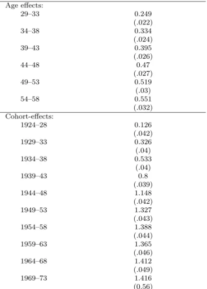
In table B.1, I regress ln(Cjt/Hjt) in a series of age and cohort dummies in
order to findφj and λt−j. All dummies are statistically significant. Figure 5 show
plots ofφj. The age profile of the relative supply of college-educated workers has a
concave shape, having a very positive slope for initial ages, as shown in Figure B.1. Figure B.2 shows plots of λt−j. The cohort profile shows an interesting S-shape.
Generations born between 1941 and 1951 experiences the highest increase in the ratio between college and high school educated workers. Nonetheless,λt−j reaches
the maximum value for the cohort born in 1969-73.
Table B.1
Estimated models for the relative supply of college-educated workers
Age effects:
29–33 0.249
(.022)
34–38 0.334
(.024)
39–43 0.395
(.026)
44–48 0.47
(.027)
49–53 0.519
(.03)
54–58 0.551
(.032) Cohort-effects:
1924–28 0.126
(.042)
1929–33 0.326
(.04)
1934–38 0.533
(.04)
1939–43 0.8
(.039)
1944–48 1.148
(.042)
1949–53 1.327
(.043)
1954–58 1.388
(.044)
1959–63 1.365
(.046)
1964–68 1.412
(.049)
1969–73 1.416
(0.56)