The evolution of the college-high school wage differential for males in Brazil: Does an increasing supply of college-educated labor explain it?

Differential for Males in Brazil: Does an Increasing

Supply of College-educated Labor explain it?

Sergio G. Ferreira

[email protected]

Department of Economics

University of Wisconsin-Madison

February 19th, 2002

I - Introduction1

Education attainment of the labor force has mildly increased in the last two decades in

Brazil. I am interested in testing if the increase in the number of workers with a college

degree has somewhat led to a downward pressure in the college wage premium. The

premium is defined as the wage difference between workers with a college degree and

workers with a high school degree.

There is recent work that examines the effects of supply changes on the returns to

education in the US, Canada and UK. The seminal work, by Lawrence Katz and Kevin

Murphy (1992) looks at movements in the college wage premium in the US from 1963 to

1987 and concludes that “it appears to be strongly related to fluctuations in the rate of

growth of the supply of college graduates”. Their model assumes perfect substitutability

among workers in different age groups as long as they have the same level of education.

Such an assumption allows them to construct an aggregate education index as a linear

combination between the “amount of education” supplied by workers of different ages.

David Card and Thomas Lemieux (NBER,2000) extend Katz & Murphy’s model to allow

imperfect substitution between workers of different ages. By measuring the impact of

changes in the supply of education (of different age groups) on the college wage

premium, they are able to estimate the elasticity of substitution between different age

groups with the same education level. Once they estimate this parameter, they are able to

calculate aggregate indexes for the total supply of high school and college workers in the

labor force that take into account the imperfect substitution between age groups. Their

estimates for the US suggest that the elasticity of substitution between different age

groups is large but finite at 4.4, while the elasticity of substitution between college and

high school labor types is in the range of 1.1 to 1.6. Results are similar for both the UK

and Canada.

My work examines the applicability of their results in a context of a developing country.

In Brazil, the college-high school wage gap for full-time male workers stays fairly flat

7% in 1988. After 1988, however, it has been fluctuating around 2.20. During the same

period, the number of workers with college education in the labor force has being

increasing relative to the number of high school workers. This paper examines how

changes in the supply of school-related labor has affected the pattern observed in the

college-high school wage gap.

I closely follow the two-step estimation method applied by Card & Lemieux (2000). The

theoretical model has a production function that uses only labor as input. However, labor

can be of two kinds: high school type and college type, combined under a CES

technology. It is straightforward to show that the college-high school wage gap for a

given age-group depends on both the aggregate relative supply of college labor in period

t, and on the age-group specific relative supply of college labor.

To do this work, I create a panel of age/time cells for the period from 1976 to 1998,

where each age/time cell contains estimates of college wage premium, college-specific

labor supply and high-school-specific labor supply. Each age-specific supply will be

measured by the number of individuals in the labor force (weighted by their respective

number of hours worked). Aggregate high school labor may not be a linear combination

of school labor at different ages, because age groups might be imperfect substitutes.

Hence, as a first step, I estimate the elasticity of substitution between age groups within

the educational group by regressing the school premium on time dummies, cohort

dummies and on the age-group specific relative supply of college labor. Based on the

estimated partial elasticity of substitution and estimated cohort-specific productivity

factors, I am able to calculate the aggregate college and high school educated labor

supply.

The second step consists of estimating the elasticity of substitution between the two

school groups by regressing the college-high school wage gap on cohort and age

dummies, a linear time trend and on the estimated time series of aggregate relative supply

of college labor.

1

One important issue is how to correctly identify changes in demand for skills from

changes in the supply of skills. Following the procedure adopted by Card & Lemieux

(2000) and Katz & Murphy (1992), among others, I assume that the effect of skill-biased

technical change on college wage premium can be summarized by a time trend. This

assumption turns out to be essential for the conclusion that school supply is an important

determinant of the college premium.

The main results of the paper are:

a) The estimation procedures reveal that the elasticity of substitution between the

two education groups is low and statistically significant. Hence, the estimation

indicates that the increasing supply of college workers over time had substantial

negative effects on the college wage gap. Depending on the proxy for the age-specific

index used, my estimates vary from 1.56 to 1.93 which are close to those observed by

Card & Lemieux (2000) for the US.

b) The estimation reveals a very small effect of relative specific college supply in the

pattern of wage gap observed by each age group (equivalent to a partial elasticity of

substitution across age groups of 16). This might be an effect of lack of specialization

in the Brazilian job market. Alternatively, this may be a result of wide changes in the

relative supply as an effect of late graduation. Estimating cohort-specific relative

supply of college-type labor which are controlled for age effects renders much

smaller partial elasticity coefficients, around 4.5.

c) The estimation reveals that the time trend of the college wag gap is significantly

positive (between 0.08 and 0.10). This might be an effect of skill-biased technology

changes, or accumulation of physical capital, if capital is a complement to skilled

labor or a substitute to unskilled labor.

My paper is the only one which actually estimate the elasticity of substitution between

age groups in Brazil. There are other studies looking at the impact of labor supply in the

school-related wage differential. Fernandes & Meneses (2002) assume three different

values for the elasticity of substitution, and estimate the impacts of demand shocks in

relative wages. The basic difference between our methods is the identification

trend. They take the inverse rout, assuming a given value for the impact of supply on the

school premium, and then estimating the impact of demand shifts on wage differentials.

The paper has five additional sections. In section II, the theoretical model is presented.

This model is based on Card & Lemieux (2000), and the only difference is that I allow

for variations in the age specific productivity factor over time. Section III presents the

empirical procedure. Section IV presents the selected sample, and explains how I

constructed the panel of wage gaps and school-related labor indexes. In addition, it

presents how the constructed series have evolved over time. Section V presents the result

of the estimations, when I do not control for the effects of late graduation in the supply of

college-type workers. In Section VI, I estimate a cohort-specific relative supply of

college-type workers that are not biased by the presence of age effects. Finally, Section

VII concludes the paper.

II – Theoretical Framework

Aggregate output depends on two CES sub-aggregates of high school and college labor:

η η

α 1/

)] (

[ _jt

j jt

t C

C =

∑

and

η η

β 1/

)] (

[ _jt

j jt

t H

H =

∑

where 1−∞<η≤ is a function of the partial elasticity of substitution σ_A between different age groups j with the same level of education (η=1−1/σ_A). Each age group has specific relative efficiency parameters, α_jtand β_jt, which vary over time. In other words, those parameters may suffer influence of cohort-specific productivity shocks (e.g.

variation in school quality).

In the limiting case of perfect substitutability across age groups, η is equal to 1 and total high-school (or college) labor input is a weighted sum of the quantity of labor supplied

I assume that the aggregate production function is also CES:

ρ ρ ρ _θ

θ 1/

)

( _{ct t ht t}

t C H

y = + , (3)

where 1−∞<ρ ≤ is a function of the elasticity of substitution σ_Ebetween the two education groups (ρ =1−1/σ_E). In this setting, the marginal product of labor for a given age-education group depends on both the group’s own supply of labor and the aggregate

supply of labor in its education category. Efficient utilization of different skill groups

requires that relative wages are equated to relative marginal products2_:

jt A jt t t ht jt t H

jt y H H H

w ) ln( / ) ln( ) ln( ) 1/ ln

ln( = ∂ ∂ = θ ρ−ηΨ + β − σ (4)

jt A jt t t ct jt t C

jt y C C C

w ) ln( / ) ln( ) ln( ) 1/ ln

ln( = ∂ ∂ = θ ρ−ηΨ + α − σ (5)

1 / 1

)

( + −

= _θ ρ _θ ρ ρ

ψ_{t ct}C_{t ht}H_t (6)

Equations (4) and (5) imply that the ratio of the wage rate of college workers in age

group j ( c jt

w ) to the wage of high-school workers in the same age group j ( H jt

w ) satisfies

to the following equation:

) / ln( / 1 ) / ln( ) / 1 / 1 ( ) / ln( ) / ln( ) /

ln( Ct Ht jt jt A E t t A jt jt

H jt C

jt w C H C H

w = θ θ + α β + σ − σ − σ . (7)

Hence, if the relative employment ratios are exogenous, equation (7) leads to a model for

the observed college-high school wage gap r_jt of workers in age group j in year t:

jt jt jt A t t E A jt jt Ht Ct H jt C jt

jt w w C H C H e

r ≡ln( / )=ln(θ /θ )+ln(α /β )+(1/σ −1/σ )ln( / )−(1/σ )ln( / )+ , (8a)

where e_jtreflects sampling variation in the measured gap and/or any other sources of

variations in age-specific wage premiums3.

2 1 1 1 1

/ /

/∂ =∂ ∂ ×∂ ∂ = −Ψ × − − = − Ψ × −

∂ _θ ρ _β η η _θ ρ η _β η

jt jt t t ht t jt jt t t ht jt t t t jt

t H y H H H H H H H H

y .

Similarly, the marginal product of college workers in age group j is ∂y_t/∂C_jt =θ_ctC_tρ−ηΨ_t×α_jtCη_jt−1. 3

According to Equation (8a), the college-high school gap for a given age group depends

on both the aggregate relative supply of college labor (C_t /H_t) in period t, and on the

age-group specific relative supply of college labor (C_jt/H_jt). When there is perfect

substitution across age groups with the same level of education, the college premium will

depend only on the aggregate relative supply of college workers, on the relative

technology shock θ_ct/θ_ht, and on the age-cohort relative efficiency parameter β_jt/α_jt.

For purposes of estimation, it is convenient to rearrange Equation (8a) in an alternative

form:

jt t t jt jt A t

t E jt jt Ht Ct

jt C H C H C H e

r =ln(θ /θ )+ln(α /β )−(1/σ )ln( / )−(1/σ )[ln( / )−ln( / )]+ (8b).

III – Econometric Method

The primary purpose of this paper is to estimate the effect of the aggregate relative

supply of college labor on the college-high school wage gap. A problem arises in the

attempt to estimate Equation (8a) because aggregate supplies of the two types of labor

(C_tand H_t) depend on the elasticity of substitution across age groups, according to

Equations (1) and (2). Following Card & Lemieux (2000), a two-step estimation provides

a method for identifying both σ_A and σ_E. In the first step, σ_Ais estimated from a regression of age-group specific college wage gaps on age group-specific relative

supplies of college educated labor, cohort effects (which absorb the relative productivity

effect , ln(β_jt /α_jt)), and time effects (which absorb the combined relative technology shock and any effect of aggregate relative supply):

jt jt jt A t

j t

jt b d C H e

r = ₋ + −(1/σ )ln( / )+ . (9)

where b_t−jare cohort dummies and d_tare time dummies. Given an estimate of 1/σ_A, the relative efficiency parameters α_jtand β_jtare easily computed by noting that equations (4) and (5) can be transformed into:

) ln( ) ln(

ln / 1 )

ln( H _{A jt ht t t jt}

jt H H

) ln( ) ln(

ln / 1 )

ln(wC_jt + σ_A C_jt = θ_ctC_tρ−ηΨ_t + α_jt , for all j and t. (11)

The left hand side of these equations can be computed directly using the first step

estimate of 1/σ_A. The right hand side can be estimated by a set of time dummies (first term) and cohort dummies (relative efficiency parameters). Given estimates of α_jt’s,

jt

β ’s and of η, it is easy to construct estimates of the aggregate supply of college and high school labor in each year (C_tand H_t).

With these estimates in hand, and some assumptions about the time series path of the

relative productivity term, log(θ_ct /θ_ht), Equation (8b) can be estimated directly. I follow the previous mentioned literature and assume that log(θ_ct/θ_ht) can be represented as a linear trend.

IV – The College Wage Premium and the Relative Supplies of College Workers by Age

In this section, I present a descriptive overview of trends in the college wage premium for

different age groups in Brazil. I also summarize data on the relative supplies of

college-educated workers by age group. The data is drawn from the Brazilian Nationwide

Household Sample (PNAD), for the years 1976 to 19984.

a. The Evolution of the College Wage Premium for Male Workers5

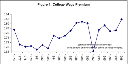
Figure 1 shows the evolution of the overall college premium for male workers since

1977. This premium is measured by the coefficient on a regression of log wage on a

college dummy and several control variables, for every year in the sample6. My estimates

4_{Data is not available for the following years: 1980, 1991 and 1994.}

5

I focus exclusively on the evolution of the college wage gap for men. I believe that this focus is appropriate, given inter-cohort changes in female labor supply that have presumably affected the age profiles of earnings for women in different education groups over the past twenty years. If women in younger cohorts accumulate more actual experience per year of potential experience than older cohorts, this will increase the measured college-high school wage even if the true college premium is fixed. Secular changes in the age profile of the college-high school wage gap may, therefore, be contaminated by these composition effects. Another reason for excluding women from the calculation of the college wage gap is that the sample female hourly labor earnings are very imprecise due to substantial variations in the number of hours worked.

6

of the college wage premiums are based on the total labor earnings (income from all jobs)

of men aged 24 to 58, living in urban areas of Brazil, who are either employed or self –

employers and are working at least 40 hours in the week of reference. In addition,

extremely low and extremely high hourly wage rates are dropped from the sample7. The

remaining sample size is 217,206 observations.

The college wage gap has been widening, but not at a constant rate over time. After

increasing substantially during the 1980’s and reaching 0.82 in 1990, the college-high

school differences of the log hourly wage has been oscillating around 0.78 during the

1990’s8. The college premium increased by 15% from 1977 to 1998, but only 1.2% from

1990 to 1998.

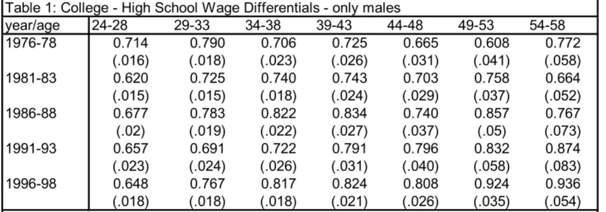
Table 1 presents my estimates of the “college wage premiums” for 5-year age groups,

taken at 5-year intervals over my sample period. The estimates are based on differences

in mean log average hourly wages between full time workers with a complete or an

incomplete college degree (i.e., at least 12 years in school) and those with a complete or

an incomplete high school degree (i.e., at least 9 and at most 11 years in school)9. The

wage gaps are estimated in separate regression models for each cohort in each “year”10.

Each model includes a dummy for college degree (defined as above), and the following

control variables: a linear age term, an indicator of self-employment, five regional

7

Wages are deflated by the GPI-FGV index, and converted to values of 1996. In 1996 values, the upper bound from 1983 to 1998 is R$ 719.00 per hour, or R$ 28.76 a week (assuming a 40 hour week). This represents respectively the percentile: 98.43%, in 1998; 98.63%, in 1997; 98.25%, in 1996; 98.77%, in 1995; 99% in 1993; 99% in 1992; 99.25% in 1990; 99.25% in 1989; 99.11% in 1988; 99.49% in 1987; 99.44% in 1986; 99.54% in 1985; 100% in 1984 and 1983. The other upper bounds, and respective percentiles in the unrestricted distribution are, in hourly terms: R$ 190.00 (99.7%), in 1982; R$ 177.00 (99.7%), in 1981; R$ 154.00 (99.78%), 1979; R$ 262.00 (99.82%) in 1978; R$ 393.00 (99.81%) in 1977; R$ 971.00 (99.71%), in 1976. The aim of such upper boundaries was to eliminate unrealistic earnings reports. Such misreporting are easily identified, since there is enormous discontinuity above the cutoff points, with the next value being as much as 100,000 larger than the chosen cut-off point. Such misreported data occurred in more than 1.75% of the sample in recent years, with a much smaller fraction for the data from the 1970s. The sample is additionally restricted by the elimination of workers earning less than R$ 6 monetary units per week (25% of the official minimum wage).

8

In 1998, a worker in the college group earned on average 2.3 times more than a worker in the high school group.

9

I can only identify a complete high school or college degree for years after 1992. It is possible that some of the changes in wage can be a result of composition within the education categories, but I do not have how to control for it.

10

dummies, and time dummies. The standard error in parenthesis is taken as weights when

estimating the model developed in Section II.

Figure 1: College Wage Premium

0.68 0.70 0.72 0.74 0.76 0.78 0.80 0.82 0.84

1976 1977 1978 1979 1981 1982 1983 1984 1985 1986 1987 1988 1989 1990 1992 1993 1995 1996 1997 1998 Estimated from regression models using sample of men with high school or college degree.

Comparisons down a column of the table show the changing college premium for a

specific age group. Older workers observe a substantial increase in the college premium

over time, especially until 1990. Wage gaps increase by 34% from 1977 to 1989 and

1.8% from 1989 to 1998. On the contrary, the wage gap is almost the same for younger

workers in 1977 and in 1998. Wage gaps increase by just 2% from 1977 to 1989 and fall

by 5% from 1989 to 1998.

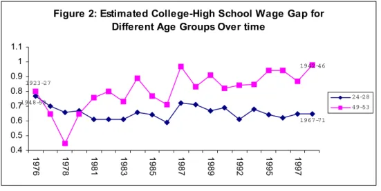
Figure 2 follows the age groups 49-53 and 24-28 over the period from 1977 to 1998. The

older group represented individuals born between 1923 and 1927, in the beginning of the

sample period, and individuals born between 1942 and 1946, in the end of the period. The

younger group represents individuals born between 1948 and 1952, in the beginning of

the sample period, and individuals born between 1967 and 1971 in the end of the period.

If age groups are perfect substitutes, the vertical distance between the two curves may

vary either because the return on experience is changing or because the idiosyncrasies of

Table 1: College - High School Wage Differentials - only males

year/age 24-28 29-33 34-38 39-43 44-48 49-53 54-58

1976-78 0.714 0.790 0.706 0.725 0.665 0.608 0.772

(.016) (.018) (.023) (.026) (.031) (.041) (.058)

1981-83 0.620 0.725 0.740 0.743 0.703 0.758 0.664

(.015) (.015) (.018) (.024) (.029) (.037) (.052)

1986-88 0.677 0.783 0.822 0.834 0.740 0.857 0.767

(.02) (.019) (.022) (.027) (.037) (.05) (.073)

1991-93 0.657 0.691 0.722 0.791 0.796 0.832 0.874

(.023) (.024) (.026) (.031) (.040) (.058) (.083)

1996-98 0.648 0.767 0.817 0.824 0.808 0.924 0.936

(.018) (.018) (.018) (.021) (.026) (.035) (.054)

OBS:

(1) College dummy coefficients in a regression model that include as control variables a linear age term, regional dummies, time dummies, and self-employment dummy. (2) The sample contains a rolling age group. For example, the 24-28 year old group in the 1976-78 sample includes individuals 23-27 in 1976, 24-28 in 1977 and 25-29 in 1978. (3) College workers are defined as workers who got at least incomplete college degree; High School workers are those who are either high school dropouts or high school graduates (exactly 11 years in school).

(4) Standard Errors in parentheses.

Equation (8a) shows that different evolutions over time of the college wage gap across

age groups could happen even in the presence of perfect elasticity of substitution across

age groups. Under the assumption of perfect substitutability between age groups, the

difference in the college premium between j and j’ at time t can be expressed by:

)

(

)

/

ln(

)

/

ln(

,'t jt jt jt jt jt jt

j

jt

r

e

e

r

−

=

α

β

−

α

β

+

−

Assume a very specific pattern for the age specific productivity factor11, such that:

j j t jt

jt β ϕ γ

α / )= ₋ +

ln( (13).

Then Equation (12) will become:

)

(

)

(

)

(

,'t j j t j t j jt jt

j

jt

r

e

e

r

−

=

γ

−

γ

+

ϕ

−

ϕ

+

−

Unfortunately, it is impossible to identify the source of such variation, if changes in the

experience returns or changes in cohort-specific “productivity” parameters without strong

assumptions. In any case, the variations in

r

−

r

11

high elasticity of substitution across age groups12. This leads to the second question I try

to answer in this paper: Do different evolutions of the school premium for different age

groups have anything to do with the evolution of the age specific supply of college labor?

Figure 2: Estimated College-High School Wage Gap for Different Age Groups Over time

0.4 0.5 0.6 0.7 0.8 0.9 1 1.1

1976 1978 1981 1983 1985 1987 1989 1992 1995 1997

24-28 49-53 1948-52

1967-71 1923-27

1942-46

b. Relative Supplies

I turn next to an overview of my estimates of the relative supplies of college-educated

labor by age group and year. I estimate relative supplies from a broad sample that

includes men and women. My estimates of relative supplies of different education groups

are based on data for men and women aged 24 to 58, who had worked as an employee or

were self-employer at least one hour in the week of reference. The sample size is

1,803,168 observations. To account for differences in the effective supply of labor by

different groups, I count the number of hours worked in the week by each worker and

weight these hours by the average wage (over all periods) of his (or her) education group.

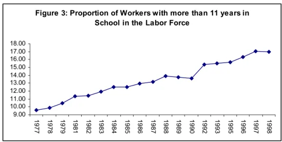
My main focus is on the evolution of the aggregate college supply over time. Figure 3

shows that there is a clear positive trend on the proportion of workers with more than

12

eleven years in school in the labor force, although this proportion is no bigger than 17%

at the end of the sample period.

Figure 3: Proportion of Workers with more than 11 years in School in the Labor Force

9.00 10.00 11.00 12.00 13.00 14.00 15.00 16.00 17.00 18.00

1977 1978 1979 1981 1982 1983 1984 1985 1986 1987 1988 1989 1990 1992 1993 1995 1996 1997 1998

I define the amount of “high school labor” of age group j in year t (H_jt) as the total

weekly hours13 worked by high school graduates or dropouts in that age range, plus the

total hours of elementary school graduates or dropouts (weighted by their wage relative

to the high school group)14. The amount of “college labor” of age group j (C_jt) is defined

as the total number of hours worked by workers with complete or incomplete college

degree15. Table 2 shows the results of calculations. The estimated relative “college labor

supplies”, in Table 2C, are used in Section V to estimate the elasticity of substitutions

between different age groups.

13

I attribute 20 hours worked for individuals who worked less than 40 hours and 40 hours for those working at least 40 hours.

14

The first group is called “incomplete high school” and the second group is the “elementary school”. Both groups are considered in the aggregate labor supply of “high school” workers, with their respective labor efficiency factors. The relative wage of the workers with complete or incomplete elementary school with respect to the wage of “high school workers” is obtained through a regression (for the whole sample period) of the log hourly real wage on a dummy for “high school workers”, regional dummies, a dummy for self employment and a squared polynomial of age. The labor efficiency factor of the “elementary school” group is 0.52. Card & Lemieux (2000) use only high school graduates or dropouts in their measure of “high school labor type”. In addition, they are able to identify high school dropouts and give respective labor efficiency weights for such group of workers, while I have to consider them with the same weight as those workers who has completed high school.

15

Table 2

A-School Supply - "High School Labor Supply" by age and year- Men and Women.

24-28 29-33 34-38 39-43 44-48 49-53 54-58

1976-78 236,713,531 146,104,657178,110,812 127,908,086 100,147,384 76,334,866 48,333,458 1981-83 299,082,493 187,009,908239,629,962 157,651,536 122,209,806 93,682,978 64,463,991 1986-88 380,783,102 259,705,668319,769,793 203,297,836 156,111,226 115,591,636 78,890,812 1991-93 243,317,801 188,706,706221,653,991 148,974,792 104,825,954 71,323,342 45,037,681 1996-98 382,365,307 329,210,492363,455,473 280,303,152 205,388,574 133,125,505 83,187,682 B-School Supply - "College Labor Supply" by age and year- Men and Women.

24-28 29-33 34-38 39-43 44-48 49-53 54-58

1976-78 50,810,740 41,364,180 24,814,440 18,517,300 12,684,040 8,245,340 4,714,280 1981-83 66,810,900 65,035,620 46,679,240 29,161,780 18,667,020 12,353,780 7,075,420 1986-88 81,617,120 93,321,780 75,724,380 51,807,620 31,262,900 17,348,500 10,413,900 1991-93 57,458,020 62,228,020 59,588,700 47,979,800 29,843,880 15,832,020 7,899,400 1996-98 88,585,800 104,679,740105,236,900 93,197,400 68,374,480 39,617,140 17,662,340 C-School Supply - Relative College Labor Supply

24-28 29-33 34-38 39-43 44-48 49-53 54-58

1976-78 0.21 0.23 0.17 0.14 0.13 0.11 0.10

1981-83 0.22 0.27 0.25 0.18 0.15 0.13 0.11

1986-88 0.21 0.29 0.29 0.25 0.20 0.15 0.13

1991-93 0.24 0.28 0.32 0.32 0.28 0.22 0.18

1996-98 0.23 0.29 0.32 0.33 0.33 0.30 0.21

OBS:

(1) High School Labor Supply == number of workers with incomplete or complete high school degree (weighted by # weekly hours) + number of workers with elementary school (weighted by # weekly hours and

by the relative wage with respect to high school wage).

(2) The average relative wage of the elementary school group (at most 8 years in school) is obtained through a regression of log real wage on age, squared age, regional dummies, and self employment dummy.

(3) College Labor Supply == number of workers with incomplete or complete college (weighted by # weekly hours) (4) Relative College Labor Supply == college labor supply : high school labor supply.

(5) The number of hours worked is represented by 20 (part time) is the individual worked less than 40 hours and 40 if the individual worked at least 40 hours.

The ratio of college labor to high school labor increases for each age group, but the

growth is significantly bigger for the older age groups. Take for example the two age

groups in Figure 4 (the same age groups as in Figure 2). The ratio of college to high

school labor increases from .21 to .24 from 1977 to 1998 for individuals aged 24-28 years

old, while the same ratio increases from .11 to .31 for the workers aged 49-5316.

If the elasticity of substitution between age groups with the same education degree were

low, a supply increase in college workers would lead to a decrease in the wage gap for

that specific age group. It is puzzling that exactly the age group that presents the higher

increase in relative supply of “college workers” is the one that experiences the higher

growth in the college wage premium. A possible explanation for this evidence is that the

elasticity of substitution between different age groups is very large. If this is true, the

different evolutions of the college wage gap across age groups only can be explained by

16

different labor-efficiency parameters for each cohort, like the one modeled in Equations

(12) to (14). In this case, the age-specific relative supply of college-educated workers will

have no effect on the evolution of age-specific college wage gaps17.

Figure 4: Relative Supply of College Workers

0.1 0.15 0.2 0.25 0.3 0.35

1976 1978 1981 1983 1985 1987 1989 1992 1995 1997

24-28 49-53 1948-52

1967-71

1923-27

1942-46

V – The Effect of Cohort-Specific Supplies on the College Wage Premium of Male

Workers18

I now turn to the estimation of the effects of the relative supply of college educated

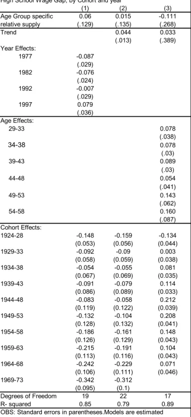
workers on the college-high school wage gap. Table 3 presents three estimations of the

partial elasticity of substitution. In Column (1), the specification includes time and cohort

dummies. In the second specification, the time dummies are replaced by a linear time

trend. In the third specification, I use a time trend, age dummies and cohort dummies as

controls.

In all three cases, the impact of the age-specific relative supply of college-educated

workers on the college wage gap is not statistically different from zero. This seems to

17

show that the partial elasticity of substitution across age groups is very high. In

regressions (1) and (2), the coefficient on the age-specific relative supply is positive.

The addition of age dummies (Column 3) changes the age-specific supply coefficient

from positive to negative, although it still not significantly different from zero. This may

happen because both the college premium and the college supply ratio increase for initial

ages, for different reasons (respectively, positive returns on experience and late college

graduation)19. Adding age dummies to the RHS in specification (3) has the effect of

controlling for this spurious relation across cohorts between college/high school ratios

and the wage gaps.

One has to be careful about the ability to identifying the age, cohort and time coefficients.

Since Age = Time – Birth Year, the identification of these effects cannot be done without

additional assumptions. In specification (1), cohort dummies capture both age effects and

cohort-specific fixed effects of the wage gap. In specification (2), the cohort dummies

will capture transitory time effects as well (for example, business cycle effects on the

college premium), since the time dummies are replaced by a time trend. In specification

(3), the life cycle shape of labor earnings is assumed to be fixed over time (captured by

the age dummy coefficients), and cohort dummies capture changes in such shape as well

as cohort-specific fixed effects and transitory time effects20.

Because specification (3) has the most complete set of controls and is the only one that

shows a negative sign, which is compatible with the theory, I assume 1/σ_A is -.11 for the

18

For all the estimations in this paper, I assume that men and women are perfectly substitutable in the labor force, with identical productivity parameters for a given age and cohort group. This assumption allows me to pool the male and female labor supply and test the impact of it on the college premium of male workers. 19

Because younger cohorts are observed only for younger ages, they will present a lower relative supply of college-educated workers, compared to cohorts observed at higher ages. At the same time, the positive return on job experience and the fact that younger cohorts are observed only for lower ages makes younger cohorts exactly the ones with a lower college-high school wage gap.

20

Table A3 in Appendix A shows the complete set of results, including the estimates of age and cohort dummies. The college wage premium reaches the maximum to cohorts born in (1944-48) and then falls continuously. This pattern shows up in all three specifications. Age dummies indicate that college premium is increasing on age, and this should be expected if the returns on experience are systematically higher for college-educated workers than for high school-educated workers. The estimated year effects absorb both the relative technology shock (θ_ct/θ_ht ) and any effect of changing aggregate supply ((1/σ −E 1/σA)ln(Ct /Ht)). The time effects are small and significant in the specifications (1) and (2),

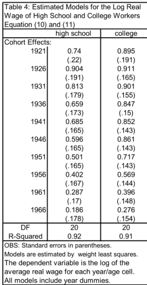
purpose of estimating the cohort-specific efficiency parameters α_jtand β_jt. Table 4 presents the estimation of equations (10) and (11). The dependent variables are,

respectively, the logarithm of the unconditional average hourly real wage of a high

school-educated worker wH_jt (column (1)) and the logarithm of the unconditional average

hourly real wage of a college-educated worker wC_jt (column (2)), net of the changes that

are related to age-specific school supply. This allows me to estimate the cohort-specific

Table 3: Estimated Models for the College - Table 4: Estimated Models for the Log Real

High School Wage Gap, By Cohort and year Wage of High School and College Workers

(1) (2) (3) Equation (10) and (11)

Age Group specific 0.06 0.015 -0.111 high school college

relative supply (.129) (.135) (.268) Cohort Effects:

Trend 0.044 0.033 1921 0.74 0.895

(.013) (.389) (.22) (.191)

Year Effects: 1926 0.904 0.911

1977 -0.087 (.191) (.165)

(.029) 1931 0.813 0.901

1982 -0.076 (.179) (.155)

(.024) 1936 0.659 0.847

1992 -0.007 (.173) (.15)

(.029) 1941 0.685 0.852

1997 0.079 (.165) (.143)

(.036) 1946 0.596 0.861

Degrees of Freedom 19 22 17 (.165) (.143)

R- squared 0.85 0.79 0.89 1951 0.501 0.717

OBS: Standard errors in parentheses.Models are estimated (.165) (.143)

by weight least squares.The dependent variable is the 1956 0.402 0.569

college-high school wage gaps shown in Table 1. Weights (.167) (.144)

are inverse sampling variances of the estimated wage gaps. 1961 0.287 0.396

All models include cohort effects. Model (3) includes age effects (.17) (.148)

as well. The years indicated when reporting the estimated year 1966 0.186 0.276

effects are the mid-points of the year intervals shown in Table 1. (.178) (.154)

DF 20 20

R-Squared 0.92 0.91

OBS: Standard errors in parentheses. Models are estimated by weight least squares.

The dependent variable is the log of the average real wage for each year/age cell. All models include year dummies.

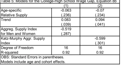
Based on estimates of 1/σ_A, α_jtand β_jt, I get estimates of the aggregate relative supply index21, which is plotted in Figure A1. Table 5 presents estimates of the second stage

models (based on Equation (8b)) that include both age-group specific relative supplies of

college labor, and the aggregate relative supply index. The relative technology shock

variable (ln(θ_ct/θ_ht)) is assumed to follow a linear trend. All the specifications include cohort and age dummies, as well as a time trend22.

In Column (1), I use the estimated aggregate supply of college and high school educated

workers as the measure of labor supply. A 10% increase in the age-specific relative

supply of college-educated workers decreases the college premium by only 0.6%, for that

21

The evolution of the estimated aggregate relative supply of college workers is plotted in Figure A1. 22

particular age-group23. This implies a very large partial elasticity of substitution of 15.9.

but the 5% confidence interval includes infinite elasticity24.

In contrast, the estimation of equation (8b) shows that the increase in the aggregate

supply of college workers substantially depressed the college premium in the last twenty

years in Brazil. A 10% increase in the relative supply of college-educated workers drives

down the college-high school wage differential by 5.2%, in the absence of non-neutral

technology changes. This is compatible to an elasticity of substitution between college

and high school workers of 1.9325.

The time trend coefficient is 0.08 and it is significant at 5%. This means that, absent the

age/cohort productivity factor and the changes in school supply, the college wage gap

would have increased on average by 8% in each 5-year period. Note that such large,

positive and significant coefficients of the time trend contrasts with the trend coefficients

in Table 3. The insignificance of the time trend in Table 3 (especially specification (3))

happens because college supply is driving down wage gaps while the skill-biased

technology changes are driving up the returns to college education.

23

Controlling for age dummies changes the coefficient on the aggregate index from -.44 to -.52, but the age-specific supply coefficient goes from -.007 to -.063.

24

Variations in the supply ratio across different ages for a given cohort does not seem to depress wage gaps. At the same time, it seems to be big enough to dominate the variations across different cohorts for a given age. In Appendix B, I replace the age-specific relative supply ratio by an estimated supply ratio that is fixed for a given cohort, and re-estimate the elasticity of substitution coefficients. The main conclusion is that, absent the age profile of the college-high school ratio, cohort variations are negatively correlated to the wage gap. The estimated impact of cohort-fixed supply on the college wage gap is -.229 (which is equivalent to a partial elasticity of substitution between age groups of 4.36). The estimate of the elasticity of substitution between school types falls to 1.56.

25

Table 5: Models for the College-High School Wage Gap, Equation 8b

(1) (2)

Age-specific -0.063 -0.07

Relative Supply (.236) (.234)

Trend 0.083 0.094

(.039) (.041) Aggreg. Supply Index -0.519

for Men and Women (.287)

Katz-Murphy Aggr. Supply -0.599

Index (.301)

Degree of Freedom 16 16

R-squared 0.92 0.92

OBS: Standard Errors in parentheses. Models include age and cohort effects.

Does the estimate of the elasticity of substitution between school groups change if I

assume infinite partial elasticity between age groups? In Columns (2), I adopt the simple

aggregation of college and high school workers across age, assuming perfect substitution

across age-groups, as done in Katz & Murphy (1992). In this case, the estimate of the

elasticity of substitution between school groups decreases slightly to 1.67.

VI – Instrumenting the College-High School Ratio

Variations of the supply ratio across different ages for a given cohort does not seem to

depress wage gaps. At the same time, it seems to be big enough to dominate the

variations across different cohorts for a given age. In this section, I replace the

age-specific relative supply ratio by an estimated supply ratio that is fixed for a given cohort,

and re-estimate the elasticity of substitution coefficients. The main conclusion is that,

absent the age profile of the college-high school ratio, cohort variations are significantly

correlated to the wage gap.

I can decompose the relative supply of college-educated workers into two components:

an age-specific component (φ_j) and a cohort-specific component (λ_t−j). This specific decomposition assumes that there is an age profile that is common across different

cohorts. The log of the relative supply of college-educated workers will become:

jt j j t jt

jt H u

C / )=λ₋ +φ +

Under this decomposition, λ_t−j is the projection of the relative supply on the cohort dummies:         = =

− ln( )/ j 0

jt jt j t H C E φ

λ (16).

Similarly, φ_jis the projection of the relative supply on the age dummies:

        =

= ln( )/ _t−j 0

jt jt j H C E λ

φ (17).

Table B.1 in the appendix shows the result of a regression of ln(C_jt/H_jt)in a series of

age and cohort dummies in order to find

^

j

φ and t−j

^

λ . All dummies are statistically

significant. Figure B1 show plots of

^

j

φ . The age profile of the relative supply of college-educated workers has a concave shape, having a very positive slope for initial ages.

Figure B.2 shows plots of t−j

^

λ . The cohort profile shows an interesting S-shape. Generations born between 1941 and 1951 experiences the highest increase in the ratio

between college and high school educated workers. Nonetheless, t−j

^

λ reaches the

maximum value for the cohort born in 1969-73.

Once I calculate t−j

^

λ , I can use it to estimate the partial elasticity of substitution between age groups, instead of using ln(C_jt /H_jt). Table 6 presents the estimation of equation (9),

modified by the presence of t−j

^ λ : jt j t A t j t

jt b d e

r = ₋ + − ₋ +

^

) / 1

( σ λ (18).

Table 6 can be compared to the results found in Table 3. The estimated partial elasticity

of substitution is 4.40 or 4.65, depending if the specification includes or not age

groups, changes across cohorts in the supply of college-educated workers has a negative

and significant impact in college wage gap26.

The next step is estimating equation (10) and (11). I assume 1/σ_A =−.227, and use this value to estimate ln(β_jt)and )ln(α_jt , respectively the age/cohort productivity factor of high-school-educated and college-educated and workers. Table 7 is the analog of Table 4

and shows the estimates of ln(β_jt) (column(1)) and ln(α_jt) (column (2)) – the cohort dummies coefficients. I use the estimates of ln(α_jt)and )ln(β_jt to calculate the aggregate supply of college-educated and high-school-educated workers, with the respective cohort

efficiency parameters.

Table 8 shows the result of the estimation of Equation (8b), analog to Table 5. Using the

cohort-specific measure of relative supply of college-educated workers, instead of the

age/time relative supply (as done in Table 5), I find that a 10% increase in cohort supply

of the college/high school ratio leads to a 2.3% decrease in cohort-specific college/high

school wage gap - when controlling for age and cohort effects27. This means that there is

a partial elasticity of substitution between age groups of 4.34. The coefficient is

statistically significant (the interval does not include zero as a possibility). This confirms

my expectation that changes in the supply of college-educated workers across age

(related to late graduation) seems to be causing the insignificant coefficients found in

Table 3 and Table 5.

26

When controlling for age effects, for example, a 10% increase in college supply for a given cohort would lead to a 2.3% decrease in college wage gap for that cohort with respect to other cohorts.

27

Table 6: Estimated Models for the College - Table 7: Estimated Models for the Log Real

High School Wage Gap, by Cohort and year - Equation (9) Wage of High School and College Workers

(1) (2) (3) Equation (10) and (11)

Cohort-specific -0.219 -0.215 -0.227 high school college

relative supply (.044) (.048) (0.04) Cohort Effects:

Trend 0.045 0.049 1921 0.459 0.551

(.007) (0.006) (.24) (.221)

Year Effects: 1926 0.669 0.623

1977 -0.094 (.208) (.191)

(.024) 1931 0.609 0.661

1982 -0.079 (.196) (.18)

(.022) 1936 0.48 0.647

1992 0.001 (.189) (.173)

(.022) 1941 0.533 0.702

1997 0.092 (.180) (.165)

(.024) 1946 0.479 0.779

Age Effects: (.18) (.165)

29-33 0.034 1951 0.42 0.68

(0.023) (.18) (.165)

34-38 0.008 1956 0.354 0.562

(0.022) (.182) (.167)

39-43 -0.004 1961 0.263 0.399

(0.022) (.186) (.171)

44-48 -0.064 1966 0.178 0.286

(0.022) (.194) (.172)

49-53 0.003 DF 20 20

(0.023) R- squared 0.94 0.96

54-58 OBS: Standard errors in parentheses.

Models are estimated by weight least squares. Cohort Effects: The dependent variable is the log of the

1924-28 -0.116 -0.131 -0.137 average real wage for each year/age cell.

(.048) (.051) (.044) All models include year dummies.

1929-33 -0.007 -0.017 0.003

(.041) (.044) (.038) Table 8: Models for the College-High School

1934-38 0.083 0.065 0.081 Wage Gap, By Cohort and Year - Equation (8b)

(.037) (.039) (.035) (1) (2)

1939-43 0.117 0.101 0.114 Cohort-specific -0.217 -0.229

(.035) (.037) (.033) Relative Supply (.046) (.035)

1944-48 0.218 0.202 0.212 Trend 0.093 0.1

(.04) (.043) (.039) (.027) (.021)

1949-53 0.213 0.195 0.208 Aggreg. Supply Index -0.604 -0.64

(.044) (.047) (.041) for Men and Women (.22) (.201)

1954-58 0.171 0.151 0.148 Degree of Freedom 22 17

(.047) (.050) (.043) R-squared 0.82 0.92

1959-63 0.13 0.114 0.104 OBS: Standard Errors in parentheses.

(.047) (.050) (.043) Model (1) includes cohort effects. Model (2)

1964-68 0.109 0.086 0.071 includes age and cohort effects.

(.051) (.054) (.046) 1969-73

Degrees of Freedom 20 23 18

R- squared 0.85 0.79 0.89

The coefficient of the aggregate supply index is equal to -0.64, meaning that a 10%

increase in the aggregate relative supply of college-educated workers leads to a 6.4% fall

in the college/high school wage gap, which is equivalent to an estimate of 1.56 for the

elasticity of substitution between college and high school workers. This is slightly

smaller than the one found in Section V28.

VII - Conclusion

In this paper, I estimate the impact on the college wage of the evolution in the relative

supply of college graduate workers in the labor force. I test such evidence in the context

of a developing country, Brazil.

My results indicate that the partial elasticity of substitution across age groups (within a

given school group) seems to be very large (around 16) when do not controlling for age

effects on labor supply. More important, the elasticity of substitution between

college-educated and high school-college-educated labor lies between 1.56 and 1.93. The coefficient of

the impact of aggregate labor supply on the college wage gap are all negative and

significant. The general conclusion is that aggregate changes in education endowments

may be contributing to reduce the huge income inequality in Brazil. This might be

happening through the negative impact of a higher contingent in the labor force of

college-educated workers on the college wage premium.

One should expect that the substitutability across school-groups should be lower than the

substitutability across age groups (for a given school group). College-educated workers

are placed in relatively high skill jobs and cannot be easily replaced by high

school-educated workers. At the same time, two college-school-educated workers with different ages

can perform the same task with approximately the same efficiency.

Comparing to the early literature, there is no similar study for Brazil, but there are lots of

studies looking at the same question for developed countries. Since my technique closely

28 _{Also, the presence of a positive (significantly different from zero) long run trend to higher college/high}

matches the one used by Card & Lemieux (2000), our results are comparable. They find

an elasticity of substitution between the two education groups between 1.1 and 1.6 when

they pool men and women together, slightly lower than mine. Their definition of the

education group is different from mine, since their high school-educated workers does

not include workers with only elementary school. My broader definition of the high

school labor equivalent makes the “college labor” and “high school labor” less

substitutable. For example, workers with less than five years in school are certainly not

replaceable by college-educated workers. So, adopting more strictly-defined education

groups could increase my estimate of the elasticity of substitution.

In addition, the partial elasticity of substitution across age-groups that they find for US is

around 4.5, which is much lower than the one I find for Brazil when I do not control for

age effects on school-related labor supply. Nonetheless, my estimates are close to theirs

when I do control for such effects.

Some important qualifications are important to my results. Demand factors may be

driving up the demand for “college workers” and consequently the college wage gap. For

example, skill-biased technology shocks can increase the demand for college-educated

labor, driving up the college wage gap. In contrast, trade liberalization might be

increasing the demand for low-skill-labor-intensive goods and decreasing the demand for

high-skill-labor-intensive goods, driving downward the college wage gap29.

Accumulation of physical capital increases the school premium if capital is complement

for skilled labor and a substitute for unskilled labor. I assume that such demand-side

effects on the wage gap are translated into a linear time trend.

Fernandes & Meneses (2002) adopt the reverse side, taking as given the impact of supply

on relative wages, and estimating impact on school premium of shifts in the labor

demand . They conclude that demand impacts on wages cannot be translated by a linear

trend because it has some sort of structural break in the 90s. They call such break “trade

technology shocks) is robust to the specification and the variables representing the age specific supply of college workers.

29

liberalization”, and relates it to an increase in the demand for high-school type workers in

the 90s.

Another qualification resides in the potential room for endogeneity bias in the results of

this paper. Enrollment decisions may be influenced by expected future college premiums.

In the presence of such endogeneity, the estimates of elasticity I found will be an upper

bound for the true elasticity of substitution parameters. Nonetheless, decisions of

enrolling in high school and college study are in general bounded by the lack of schools

in Brazil, especially during the period covered in the paper. Hence, I suspect that changes

in the employment ratio reveal rather changes in the supply of undergraduate courses

(due to deregulation of educational sector) than a result of individual choice to invest

more in human capital. If this interpretation is correct, endogeneity will be a minor issue

here.

Bibliography:

Card, David and Thomas Lemieux – “Can Falling Supply Explain the Rising Return to

College for Younger Men? A Cohort-Based Analysis – NBER Working Paper 7655 –

April 2000.

Katz, Lawrence and Kevin Murphy. “Changes in Relative Wages, 1963-1987: Supply

and Demand Factors”, Quarterly Journal of Economics 107, 1992.

Meguir, Costas and Edward Whitehouse. “The Evolution of Wages in the United

Kingdom: Evidence from Micro Data”. Journal of Labor Economics, 1996, vol.14, no. 1.

Menezes, Naércio, Reynaldo Fernandes and Paulo Piccheti. “The Distribution of Male

Wages in Brazil: some stylized facts.”mimeo. Universidade de São Paulo. 1998.

Menezes, Naércio and Reynaldo Fernandes – “Escolaridade e Demanda Relativa por

Trabalho: Uma Avaliação para o Brasil nas Décadas de 80 e 90”- Universidade de São

Paulo. 2002.

Moreira, Mauricio and Sheila Najberg. “O Impacto da Abertura Comercial sobre o

Emprego: 1990-1997”. In “ A Economia Brasileira nos Anos 90”. By Giambiagi, Fabio

APPENDIX A – Main Estimations

Table A1- Sample Selection - by Birth Year

year/age 24-28 29-33 34-38 39-43 44-48 49-53 54-58

1976-78 1949-53 1944-48 1939-43 1934-38 1929-33 1924-28 1919-23 1981-83 1954-58 1949-53 1944-48 1939-43 1934-38 1929-33 1924-28 1986-88 1959-63 1954-58 1949-53 1944-48 1939-43 1934-38 1929-33 1991-93 1964-68 1959-63 1954-58 1949-53 1944-48 1939-43 1934-38 1996-98 1969-73 1964-68 1959-63 1954-58 1949-53 1944-48 1939-43

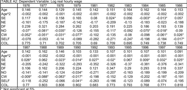
TABLE A2: Dependent Variable: Log real hourly wage

1976 1977 1978 1979 1981 1982 1983 1984 1985 1986

Age 0.146 0.144 0.129 0.145 0.142 0.151 0.164 0.162 0.164 0.153

Age^2 -0.002 -0.002 -0.001 -0.002 -0.001 -0.002 -0.002 -0.002 -0.002 -0.002

SE 0.117 0.149 0.158 0.165 0.08 0.024* 0.056 -0.003* -0.013* 0.057

NE -0.161 -0.175 -0.187 -0.142 -0.17 -0.209 -0.13 -0.183 -0.023 -0.188

DF 0.239 0.321 0.284 0.262 0.203 0.191 0.225 0.186 0.193 0.139

NO -0.07* -0.081* -0.035* -0.126 -0.155 -0.117 -0.092 -0.075* -0.018* -0.09 CW -0.052* -0.051* -0.031* -0.077* -0.102 -0.135 -0.08 -0.098 -0.061* 0.026* SELF -0.078 -0.053 -0.14 -0.089 -0.282 -0.271 -0.247 -0.198 -0.184 -0.017*

COL. 0.775 0.71 0.702 0.705 0.69 0.709 0.695 0.749 0.738 0.749

1987 1988 1989 1990 1992 1993 1995 1996 1997 1998

Age 0.142 0.162 0.146 0.103 0.133 0.107 0.101 0.107 0.101 0.091

Age^2 -0.001 -0.002 -0.002 -0.001 -0.001 -0.001 -0.001 -0.001 -0.001 -0.001

SE 0.026* 0.062 -0.023* -0.014* 0.027* -0.02* 0.067 0.009* 0.032* 0.025*

NE -0.205 -0.242 -0.322 -0.293 -0.352 -0.326 -0.37 -0.381 -0.376 -0.341

DF 0.106 0.162 0.206 0.224 0.121 0.347 0.29 0.293 0.318 0.337

NO -0.141 -0.141 -0.124 -0.034* -0.271 -0.207 -0.163 -0.189 -0.199 -0.209 CW -0.009* -0.088* -0.083* -0.017* -0.198 -0.152 -0.129 -0.202 -0.187 -0.191 SELF -0.118 -0.252 -0.066 -0.041* -0.263 -0.186 -0.123 -0.089 -0.074 -0.195

COL. 0.77 0.803 0.808 0.802 0.683 0.773 0.793 0.768 0.771 0.818

Table A3: Estimated Models for the College -High School Wage Gap, by Cohort and year

(1) (2) (3)

Age Group specific 0.06 0.015 -0.111

relative supply (.129) (.135) (.268)

Trend 0.044 0.033

(.013) (.389)

Year Effects:

1977 -0.087

(.029)

1982 -0.076

(.024)

1992 -0.007

(.029)

1997 0.079

(.036) Age Effects:

29-33 0.078

(.038)

34-38 0.078

(.03)

39-43 0.089

(.03)

44-48 0.054

(.041)

49-53 0.143

(.062)

54-58 0.160

(.087) Cohort Effects:

1924-28 -0.148 -0.159 -0.134

(0.053) (0.056) (0.044)

1929-33 -0.092 -0.09 0.003

(0.058) (0.059) (0.038)

1934-38 -0.054 -0.055 0.081

(0.067) (0.069) (0.035)

1939-43 -0.091 -0.079 0.114

(0.086) (0.089) (0.033)

1944-48 -0.083 -0.058 0.212

(0.119) (0.122) (0.039)

1949-53 -0.132 -0.104 0.208

(0.128) (0.132) (0.041)

1954-58 -0.186 -0.161 0.148

(0.126) (0.129) (0.043)

1959-63 -0.215 -0.191 0.104

(0.113) (0.116) (0.043)

1964-68 -0.242 -0.229 0.071

(0.106) (0.111) (0.046)

1969-73 -0.342 -0.312

(0.095) (0.1)

Degrees of Freedom 19 22 17

R- squared 0.85 0.79 0.89

OBS: Standard errors in parentheses.Models are estimated by weight least squares.The dependent variable is the college-high school wage gaps shown in Table 1. Weights are inverse sampling variances of the estimated wage gaps. The years indicated when reporting the estimated year

Figure A1: Relative Aggregate College Labor Supply 0.2 0.22 0.24 0.26 0.28 0.3 0.32 0.34 0.36

1977 1982 1987 1992 1997

Appendix B – Instrumenting the College-High School Ratio

Table B1: Estimated Models for the Relative Supply of College-Educated Workers Age Effects: 29-33 0.249 (.022) 34-38 0.334 (.024) 39-43 0.395 (.026) 44-48 0.47 (.027) 49-53 0.519 (.03) 54-58 0.551 (.032) Cohort Effects: 1924-28 0.126 (.042) 1929-33 0.326 (.04) 1934-38 0.533 (.04) 1939-43 0.8 (.039) 1944-48 1.148 (.042) 1949-53 1.327 (.043) 1954-58 1.388 (.044) 1959-63 1.365 (.046) 1964-68 1.412 (.049) 1969-73 1.416 (.056)

OBS: Standard errors in parentheses.Models are estimated by weight least squares.The dependent variable is the college-high school wage gaps shown in Table 1. Weights are inverse sampling variances of the estimated wage gaps.

Figure B.1: Age Profile of the Relative Supply

0.05 0.06 0.07 0.08 0.09 0.10

26 31 36 41 46 51 56

Age

Figure B2: Cohort Profile of the Relative Supply

0.05 0.07 0.09 0.11 0.13 0.15 0.17 0.19 0.21 0.23 0.25

1921 1926 1931 1936 1941 1946 1951 1956 1961 1966 1971