Roberto Ellery Jr.** Victor Gomes*** Adolfo Sachsida****
Summary: 1. Introduction; 2. Data set; 3. Cycles; 4. The standard growth model; 5. The indivisible labor model; 6. Findings from sim-ulation; 7. Conclusions.
Key words: real business cycles; aggregate fluctuations; technology shocks.
JEL codes: E32 and O41.
This paper documents the empirical relationship in postwar Brazil between the GNP and other key variables such as consumption, in-vestment, productivity and hours worked. Since many of those series were not available to Brazil we also had to build a data-set, which includes consumption of non-durables, capital and hours worked. We use two filters to extract the cycles (the usual Hodrick-Prescott filter and a band-pass filter); this procedure was taken to avoid conclusions that depend too much on the filter in use. The paper also provides simulations of two dynamic general equilibrium models (the stan-dard RBC model and the indivisible labor model) and tries to match the facts of the artificial economy with those of the actual economy. We show that the basic models fail to replicate some of the observed facts.
Este artigo documenta as rela¸c˜oes entre o PNB e outras vari´aveis macroeconˆomicas, tais como: consumo, investimento, produtividade e horas trabalhadas, observadas no Brasil. Desde que muitas destas s´eries n˜ao estavam dispon´ıveis constru´ımos uma base de dados que inclui consumo de n˜ao-dur´aveis, capital e horas trabalhadas. Para extrair o ciclo utilizamos dois filtros (o filtro Hodrick-Prescott e um filtro do tipo band-pass); este procediment foi tomado para evitar conclus˜oes que dependessem do filtro utilizado. O artigo tamb´em apresenta simula¸c˜oes de dois modelos de equil´ıbrio geral dinˆamico (o modelo b´asico de ciclos reais e o modelo com trabalho indivi´ıvel) e compara os fatos gerado pelos modelos com os observados para a economia brasileira. Este exerc´ıcio mostra que os modelos utilizados n˜ao s˜ao capazes de reproduzir alguns dos fatos observados.
*This paper was received in Nov. 2000 and approved in Dec. 2001. We would like to thank F´abio Kanczuck, Arilton Teixeira, Pedro C. Ferreira, Marcelle Chauvet, Ricardo O. Caval-canti, Samuel Pessoa, Jo˜ao V. Issler, Eust´aquio J. Reis, Elcyon Caiado, Jos´e H. Bizarria, and specially Mirta S. Bugarin, as well as the seminar participants at the II Encontro EPGE-FGV/FEA-USP de Macroeconomia, Institute for Applied Economic Research and University of Brasilia for their comments and suggestions. The usual disclaimer applies.
**Institute for Applied Economic Research (Ipea) and University of Bras´ılia (UnB). ***Department of Economics/UnB.
****Catholic Univesity of Bras´ılia (UCB).
1. Introduction
A central concern of the new-classical macroeconomics is the relationship between theory and facts. Such a concern can be traced back to the beginning of the century when a commom criticism of the neoclassical economy was the lack of empirical counterparts for the theoretical predictions. From those years the use of quantitative methods to evaluate actual economies and the results from theoretical models have developed in an incredible way. Most of those developments were in the econometric field, at least until the advent of the new-classical macroeconomics and its real business cycle (RBC) models.
The use of calibrated equilibrium models to reproduce the properties of duration and amplitude of actual economies has been present in economics for a long time;1
however, the modern techniques of using dynamic general equilibrium models to simulate key features of actual economies began with Kydland and Prescott (1982). In this seminal paper they calibrate a modi-fied version of the basic equilibrium growth model in order to replicate basic properties of the American economy. Their point is that the inclusion of time to build would generate a model where the persistence of the output would match the persistence of the American output. By using this kind of pro-cedure to test models they were starting a new approach to explain facts in actual economies.
In the very heart of the new approach was the idea that calibrated the-oretical models should be able to replicate key facts of actual economies. In this sense any model consistent with optimum behavior of firms and individ-uals may be tested through the RBC approach, there is no reason whatsoever to avoid hypotheses that are strange to the new-classical macroeconomics, as long as the hypothesis is consistent with a dynamic general equilibrium (DGE) model.
From this perspective the name “real business cycle” may not be the most appropriate to describe the new methodology, for some authors in the field are calibrating and simulating models with interesting nominal properties: recently even papers presenting nominal rigidities have been incorporated into the RBC analysis (see, for example Chari, Kehoe & McGrattan, 2000). The
1
only practical restriction on incorporating new hypotheses into the calibrated DGE models is computational. Furthermore, the new hypothesis should also help to explain the cyclical phenomena.
The principle that theoretical models should have some empirical coun-terpart can be illustrated in this passage from Ragnar Frisch, mentioned by Kydland and Prescott (1991): “theory, in formulating abstract quantitative notions, must be inspired to a larger extent by the technique of observation. And fresh statistical and other factual studies must be the health element of disturbance that constantly threatens and disquiets the theorist and pre-vents him from coming to rest on some inherited, obsolete set of assumptions. (Ragnar Frisch, in his editorial statement introducing the first issue of Econo-metrica, 1933)”.
Frisch also points out that in the set of quantitative techniques applied to the economic analysis is the business cycle theory. In this sense the mod-ern models inherited Frisch’s apprehension over the empirical bases to justify theoretical constructions. In models of cycles it is natural that the main fo-cus is related to the cyclical properties of a given economy. Of course, if one wants to deal with cycles, one should have a definition of cycles. To provide such a definition Stock and Watson (1999), and also Diebold and Rudebusch (1999), have quoted Burns and Mitchell (1946:3): “A cycle consists of expan-sions occurring at about the same time in many economic activities, followed by similar general recessions, contractions, and revivals which merge into the expansion phase of the next cycle; this sequence of changes is recurrent but not periodic; in duration business cycles vary from more than one year to ten or twelve years; they are not divisible into shorter cycles of similar character with amplitudes approximating their own”.
Stock and Watson (1999) stress that the two main empirical questions are how to identify historical business cycles and how to quantify the comovement of a specific time series with the aggregate business cycle.
the facts in this paper and follows the procedures proposed by Cooley and Prescott (1995). Moreover, simulations of the calibrated models are provided and the results are compared with the Brazilian facts.
Section 2 describes a data set compatible with business cycle analysis. Section 3 shows the second moments of the Brazilian cycle. Section 4 presents a calibrated version of the basic RBC model, while section 5 extends the model in order to incorporate the indivisible labor hypothesis. Section 6 discusses the cyclical properties generated by the simulated models and compares them with the cyclical properties of the Brazilian economy. Finally, section 7 presents some conclusions and suggestions for future researches.
2. Data Set
2.1 Gross national product
The gross national product series was obtained from the national account-ing tables. From 1947 to 1986 it was calculated by the Brazilian Institute of Economics (IBRE/FGV), a department of the Getulio Vargas Foundation in Rio de Janeiro (FGV). In 1986 the government decided to calculate the na-tional accounting tables by itself through the Brazilian Institute for Geography and Statistics (IBGE), which is an official institute.
While those changes implied some modifications in the methodologies to account for the GNP, they were not so relevant as to spoil the complete series. Some of the most relevant problems arising from them will be discussed in this section.
We use the GNP rather than the more traditional gross domestic product (GDP) in order to create a data set compatible with the real business cycle research. Since most models of RBC deal with closed economies, the GNP is more appropriate than the GDP. Figure 1 displays both series from 1947 to 1998.
2.2 Consumption
The original series of final consumption comes from the national account-ing tables and is composed of the consumption of the families and the con-sumption of the government. While the government’s concon-sumption can be used as it appears on the national accounting tables, the consumption of the family must be adjusted in order to match the series consistent with the busi-ness cycles analysis.
Two problems in the consumption of the families series deserve special attention. The first is related to the inclusion of changes in the inventories, which have been counted as consumption since 1986. The second problem is that the national account tables fail to provide a series specifically for consumption of non-durables. While it is true that other problems are related to this series,2
those two were selected because they are particularly relevant to the business cycle analysis.
Figure 2 shows the total consumption, family consumption and govern-ment consumption from 1947 to 1998. Those series were extracted directly from the national accounts data, so they present all the problems described
2
above. Throughout this section we are going to separate the series, from the stock problem and then we will try to identify the consumption of non-durables.
Consumption of the families
Changes in inventories
The problem of separating the changes in inventories from consumption arose in 1986, as a consequence of the inclusion of the changes in the inventories in the final consumption series. Before that year the national account was elab-orated by IBRE/FGV. In 1986 this task was transferred to IBGE. The official institute suppressed the series of changes in inventories from the national ac-count tables, since consumption was done by residual. Thus, the suppressed value was put into the consumption series.
Consumption of non-durables
While the problem with the changes in inventories was not so hard to solve and of minor consequence, the question of how to identify the consumption of non-durables in the total consumption series is a much harder one. Actually, from 1947 to 1969 one cannot even try to solve this problem, since there is not a regular series of input-output matrix.
Attempts to put together the very sparce information on these years and to use some interpolation technique are bound to fail as a consequence of the structural changes that the Brazilian economy was subject to in this period. It is almost a consensus that those were the years of Brazilian industrialization. It is widely known that Brazil was a mainly agricultural country in the 1940s and now it is a heavily industrialized one. Of course, those changes were of huge impact on the composition of the consumption.
In the period from 1970 to 1989 the situation improves slowly. First, besides the growing industrialization in the 1970s, it is arguably fair to assume that there were fewer changes in the composition of consumption in these years. The changes involved in a long period of growth are far less dramatic than the ones associated with the transition from a rural to an urban economy. Data from the input-output matrix for the years 1970 to 1980 show that the share of consumption of non-durables moved from 0.62 to 0.61. This fact clearly supports the stability assumption.
The other good thing is that there are a published input-output matrix3
for the years 1970, 1975, 1980, 1985, and 1990. With these matrices one can calculate the share of the consumption of durables over total consumption for each year. Taking into account the stability of these shares, it is possible to use interpolation to provide a value in the years without a matrix. To do this the following method was used:
a) find the durable share in each year with an input-output matrix;
b) use a linear interpolation to fill out the series in the years with no data;
c) create a shock with zero mean and the same standard deviations as the actual series;4
3
The matrix has 81 commodites and 42 activities.
4
d) calculate a new share, adding the interpolated to the shock, i.e.,
share=interpolated+shock;
e) multiply the share by the total consumption;
f) find the consumption of non-durables as a residual, i.e., non-durables=total-durables.
This procedure was able to generate a non-durable consumption series from 1970 to 1990; from this last year on, it was possible to use the annual input-output matrix to obtain the consumption of non-durables. Figure 3 shows the consumption of non-durables series.
Besides being of extreme importance to calibrate consumption in Brazil, the series of consumption of non-durables will be very useful to build a series of capital for Brazil. As one knows, to be consistent with the real business cycle analysis, consumption of durables should be added to investment (Cooley & Prescott, 1995).
Government consumption
other series it has been deflated by the implicit GDP deflator. Figure 4 dis-plays the series.
The government consumption includes durable as well non-durable goods. This is a problem because we cannot separate the consumption into durables and non-durables. We cannot apply the same methodology of the consump-tion of the families to the government consumpconsump-tion because the naconsump-tional ac-counting system does not provide a support to separate the consumption of durables from that of non-durables. This problem was of somewhat minor consequence due to fact that most of the government consumption came from services.5
2.3 Investment and capital
The investment series comes directly from the national account tables. The only correction was to sum up the changes in inventories from 1986 to 1998. The procedure to obtain the value on the changes in inventories was described in section 2.2.1. Also an expanded investment series was created
5
to account for the consumption of durables. Figure 5 displays the complete investment series and the investment plus consumption of durables from 1970 on.
Capital stock
To create a series of capital stock one may use the expanded investment
series and the recursive formulaKt+1= (1−δ)Kt+It, whereK is the capital stock, δ is the depreciation rate and I is the investment. However simple this approach may look, it is not straightforward when one tries to use it.
First, there are no initial values for the capital stock, neither IBRE/FGV nor IBGE provides an official estimate. Consequently, without a non-durables consumption series, the investment will be underestimated, with implications
for the calibration of the discount rate. Finally, there is not a good estimate of the value ofδ, not even a common range of values.6
Since the work on consumption was able to create a non-durables con-sumption series only for the period between 1970 and 1998, the capital series
6
will only cover those years. The lack of a good estimate of the initial capital stock and of the depreciation rate induced the choice of an iterative method to find the capital series. While this method has no econometric support, it
ends up being as arbitrary as any method which depends on an initial value or a depreciation rate parameter, with the advantage that it is fully compatible with the calibration technique. The capital series was calculated according to the following methodology:
a) at the steady state the depreciation rate is defined by δ = I
K + 1−(1 +
n)(1 +x), wherenis the growth rate of the population andxis the mean of the GDP per capita growth rate;
b) provided an initial guess to I
K, nand x are calculated from the series on GDP and population;7
c) with these values δ is calculated according to the expression above;
d) from the ruleKt+1= (1−δ)Kt+It, the values ofKt+1are calculated; this
procedure is followed for the calculation of the whole series of capital;8
e) then the mean values of It
Kt are found; if they match the guess in (b) up
to a previous criteria, the algorithm is stopped; otherwise, the new value
is used as a guess and a return is made to (c).
To refine the procedure, the series was divided in three periods, the first covers the years between 1970 and 1980, the second goes through the 1980s, and the third goes from 1990 to 1998. The reason for making this partition
is that the depreciation rate may be changing over time. Figure 6 shows the resulting capital series for Brazil:
7
To provide the initial guess one may use the observed investment-output ratio; this value is near 0.18.
8
As one can see, the series accounts for the fast growth in the 1970s, the so-called Brazilian economic miracle, and for the great recession of the 1980s, the “lost decade”, following the external debt crisis in 1982.
2.4 The labor market
In this subsection we document the relevant facts about the aggregate labor market. We take several measures of hours worked and productivity at some sample periods. The data about the labor market are separated into two parts: one for the time that households spend on market activities and the other for the hours worked. As in the other series, there is a lack of data.9
Time on market activities
The data about the time given by households to market activities was computed from the two households-survey type. We extracted these data from
9
the Brazilian decennial census and from Pnad (National Survey by Household Sample), both from IBGE. The data coverage is from 1970 to 1996, with missing points in 1974, 1975, 1991, and 1994.
To analyze these data we made used a methodology proposed by McGrat-tan and Rogerson (1998). The problem with these data is that: there is one input for each range of hours worked by households. In practice, the fields and categories of these records are as follows:
• E39= employed up to 39 hours per week;
• E40-48= employed 40-48 hours per week;
• E49= employed 49 or more hours per week;
• E = total of Informants per survey;
• A = work force;
• N = total population;
• H = (30E39+ 44E40-48+ 54E49)(A/E), where H is hours;
• H/A = hours per worker;
• H/N = hours per capita.
To construct the aggregate series we computed weighted sums. For each aggregate class, the weight for each particular group’s population is the frac-tion of the total populafrac-tion that the group represents. For example, in the first class of hours, less than 39, we find the appropriate weight looking to the irregular set of hours worked in the surveys.
The main fact for this data set is that the number of weekly hours of market work per capita has changed very little over the period, i.e., it has been roughly constant since 1970. From the mean of total of hours per worker we find that households spend 1/3 of their time engaged in market activities and 2/3 of their time in non-market activities.
Hours worked, employment, and productivity
while Fiesp covers only the industrial activity in S˜ao Paulo.10
On the other hand, while PIM-DG covers only the period from 1985 to 1998, Fiesp provides data from 1975 to 1998.
The data on employment also came from the PIM and Fiesp databases. We report these data for the same period as hours worked. Finally, productivity, in fact, is the labor productivity. The productivity of labor is defined as the output (GNP) per hours worked for both series, PIM-DG and Fiesp.
3. Cycles
A common property of economics series is that they display cycles. At least this is the assumption behind RBC analysis. In this section we will describe the main features of the cycles in Brazil. To achieve our objectives we are going to filter the series from frequencies that are too high or too low to be classified as part of the business cycle.11
We begin our study using a filter proposed by Hodrick and Prescott (1997), the so-called HP-filter. Among the reasons for using this filter lies the fact that it is the standard filter in use on real business cycle literature (Cooley & Prescott, 1995), and that, being widely used, there is a lot of research dealing with the advantages and problems of using such a filter. Furthermore, it has an easy computational implementation, with codes provided for a wide range of software.
Although it is the most popular tool to separate cycles, trends and ir-regular movements present in the series, the HP-filter has been subject to some criticism. A variety of problems has been detected, suggesting that the filter may be unable to perform well (Baxter & King, 1999). The potential problems with the HP-filter are more evident when one tries to filter annual data.12
Since those are the kind of data we are dealing with in this paper, we chose to provide evidence with another filter, besides the HP. This was the band-pass filter proposed by Baxter and King (1999).
10
The state of S˜ao Paulo accounts for nearly 70% of the Brazilian industrial production.
11
Too high a frequency may be associated with irregular movements in the series, while too low a frequency is associated with movements over long periods, which are realated to trends.
12
3.1 The HP-filter approach
The HP is the standard filter in the RBC literature. Many studies in the field use this filter as a tool to separate cycles from other movements present in an economic series. In this section we will present the main properties of the HP-cycles, defined as the cycle obtained through the Hodrick and Prescott procedure.
As we were unable to create a complete set of series fully consistent with the real business cycle theory for the whole period, from 1947 to 1998, the section will be divided into two subsections. The first will present the cyclical properties of the whole sample, while the second will concentrate on the period from 1970 to 1998. For both samples we are going to set the smoothing parameter of the HP-filter as 100.13
Cycles from 1947 to 1998
As a consequence of industrial policies with active government participa-tion, Brazil, a rural country in 1947, became a heavily industrial country in 1998. Of course this strong-state presence shows its effects on the Brazil-ian cycle. In particular, one may observe the high correlations between the government spending and the GNP. Figure 7 displays the GNP cycle.
13
As one may conclude from figure 7, the Brazilian GNP clearly displays cycles. Moreover, there is a somewhat clear pattern beginning in the 1960s and extendeding up to the 1990s. The cycle is characterized by high peaks at intervals of 10 years. Each peak is followed by depressions, in a clearly recursive pattern. The most recent peaks may be associated with the expan-sion policy during the government of president Kubtischek in the 1950s, the Brazilian economic miracle in the early 1970s, the Cruzado Plan in the middle 1980s and the Real Plan in the 1990s. The external debt crisis in 1982 and the default on the internal debt in 1990 are related to two of the greatest Brazilian depressions, as well as the economic adjustment implemented by the military government in 1967, which also produced a depression. The basic statistics of the Brazilian cycle are described in table 1. For any given data series, we first take logarithms and then use the HP-filter to remove the trend.
Table 1
Cyclical behavior of key variables: 1947-98
Variable σx% σx/σGN P corr(x−1,GN P) corr(x,GN P) corr(x+1,GN P)
GNP 4.47 1.00 0.6934 1.0000 0.6934
CONS 4.75 1.06 0.6438 0.8881 0.5766
INV 11.27 2.51 0.4800 0.7280 0.5323
INVF 10.46 2.33 0.4677 0.6983 0.5799
GOV 7.49 1.67 0.3719 0.6141 0.6106
EXP 12.13 2.71 0.2251 0.2020 0.1037
IMP 16.01 3.57 0.3206 0.3979 0.3427
Obs.: The variables refer to: CONS, personal consumption; INV, gross domestic investment; INVF, fixed investment; GOV, government purchases of goods and services; EXP, exports of goods and services; IMP, imports of goods and services.
A feature of particular interest in the Brazilian cycle is the high volatility of the series. The ratio of 1.06 between the standard deviation of consumption and GNP is higher than one would expect from permanent income theory. Of particular interest is the high correlation between the consumption of the government and the GNP. It is a sign of the huge-state participation in the Brazilian economy.
Investment has a higher volatility than GNP (figure 10). Also it is strongly pro-cyclical. The investment in fixed capital is less volatile than total invest-ment. This suggests that the changes in inventories are more volatile than the investment.
Cycles from 1970 to 1998
Since we were not able to build the consumption of non-durables series for the entire period from 1947 to 1970, the previous section fails to be fully compatible with RBC analysis. The solution is to create new models com-patible with the data available for Brazil or to work with a smaller but fully compatible sample.
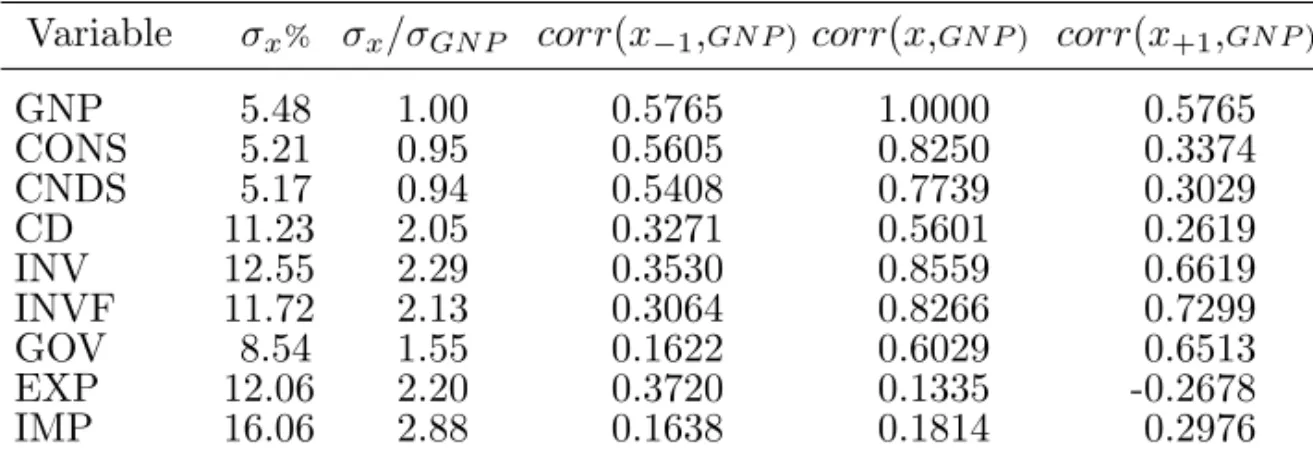
Table 2 displays the facts of the key variables for the period between 1970 and 1998. Note that, beside the even higher volatility, the facts are very similar to the ones displayed in table 1.
Table 2
Cyclical behavior of key variables: 1970-98
Variable σx% σx/σGN P corr(x−1,GN P) corr(x,GN P) corr(x+1,GN P)
GNP 5.48 1.00 0.5765 1.0000 0.5765
CONS 5.21 0.95 0.5605 0.8250 0.3374
CNDS 5.17 0.94 0.5408 0.7739 0.3029
CD 11.23 2.05 0.3271 0.5601 0.2619
INV 12.55 2.29 0.3530 0.8559 0.6619
INVF 11.72 2.13 0.3064 0.8266 0.7299
GOV 8.54 1.55 0.1622 0.6029 0.6513
EXP 12.06 2.20 0.3720 0.1335 -0.2678
IMP 16.06 2.88 0.1638 0.1814 0.2976
Obs.: The variables refer to: CONS, personal consumption; CNDS, consumption of nondurables goods and services; CD, consumption of durable goods; INV, gross domestic investment; INVF, fixed investment; GOV, government purchases of goods and services; EXP, exports of goods and services; IMP, imports of goods and services.
Personal consumption displays a contemporaneous cross-correlation with the GNP of 0.8250, and a standard deviation of 5.21. This shows that the standard deviation of consumption corresponds to roughly 95% of the stan-dard deviation of GNP.
Table 2 also shows that the standard deviation of consumption of non-durables and services is 5.17%, while the standard deviation of consumption of durable goods is 11.23%; the consumption of durables is much more volatile than the GNP and the total personal consumption. The consumption of non-durables and services has a cross-correlation of 0.7739 with the GNP and the consumption of durables has 0.5601.
Those facts seem to support the theory that Brazilian consumers are re-stricted to finance their consumption over the business cycle. Particularly, the high volatility of the consumption of non-durables, close to the GNP volatility, is a sign in this direction.
Hours, employment and productivity
Now, we turn our attention to the hours worked time series. Table 3 contains a summary of statistics for annual Brazilian data. Again we are working with data from PIM-DG and Fiesp. The variables for both surveys are hours worked (h), productivity (w), and employment (n).
For each variablej, we report the following statistics: the percentual stan-dard deviation, the stanstan-dard deviation relative to that of output σj/σy, and the correlation with output corr(j, y). We also report the relative standard deviation of hours to that of productivityσh/σw, and the correlation between hours and productivitycorr(h, w).
Table 3
Cyclical properties of labor market time series
Variable %S.D.σj/σGN P corr(j,GN P)σh/σw corr(h, w)
PIM (1985-98)
·Hours worked (j =h) 5.57 1.030 0.5376 1.05 -0.508
·Productivity (j =w) 5.27 0.978 0.4542 ·Employment (j=n) 5.13 0.952 0.4106 FIESP (1975-98)
·Hours worked (j =h) 7.15 1.440 0.6996 1.40 -0.719
·Productivity (j =w) 5.11 1.020 -0.0075 ·Employment (j=n) 5.53 1.110 0.4995
Table 3 displays the standard business cycle facts. All variables are pos-itively correlated with output. Hours worked are slightly more variable than output in PIM data and 44% more variable than output in Fiesp data. We could also verify this fact in figures 13 and 14. Variance of hours is higher than GNP. Figures 15 and 16 show respectively that employment fluctuates a little below the output in PIM data and 11% above the output in Fiesp data.
Analyzing the basic statistics for employment we note a great similarity between hours worked and employment. The variability of hours to employ-ment,σh/σn, is 1.03 (PIM) and 1.44 (Fiesp) and the correlation between hours and employment is 0.9835 for PIM data and 0.9427 for Fiesp data (figures 15 and 16).
3.2 The Band-pass filter approach
Here we describe the main statistics for the key macroeconomic variables using the band-pass filter.14
This procedure was built by Baxter and King
14
(1999) using the theory of spectral analysis of time series data. The height of the spectrum at a certain frequency corresponds to fluctuations of the periodicity that corresponds (inversely) to that frequency. Thus the cyclical component can be thought of as those movements in the series associated with periodicity within a certain range of business-cycle durations. We chose the frequencies associated with periods in the range from one to eight years. The choice was made in order to be compatible with the Burns and Mitchell (1946) classification of cyclical movements. According to this methodology, the ideal band-pass filter would preserve these fluctuations but would eliminate all other fluctuations, both the high frequency fluctuations associated, for example, with measurement error and the low frequency fluctuations associated with trend growth.
The ideal band-pass filter cannot be implemented in finite data sets be-cause it requires an infinite number of past and future values of the series; however, a feasible (finite-order) filter can be used to approximate this ideal filter. Baxter and King (1999) show that the feasible band-pass filter is based on a 12 quarters or three years centered moving average, where the weights are chosen to minimize the squared difference between the optimal and approxi-mately optimal filters. We are using the three years centered moving average specification. In table 4 we show the cyclical properties of key macroeconomic variables filtered with the band-pass filter.
Table 4
Cyclical behavior of key variables: 1970-98
Variable σx% σx/σGN P corr(x−1,GN P) corr(x,GN P) corr(x+1,GN P)
GNP 4.97 1.00 0.4971 1.000 0.4504
CONS 4.43 0.89 0.4947 0.8191 0.1627
CNDS 4.89 0.98 0.4960 0.7696 0.1149
CD 9.91 1.99 0.0957 0.2832 0.2479
INV 12.63 2.54 0.3202 0.8733 0.5530
INVF 11.65 2.34 0.2753 0.8697 0.6675
GOV 8.40 1.69 0.0483 0.5965 0.7290
EXP 13.29 2.67 0.4450 0.0975 -0.3595
IMP 16.01 3.22 0.1093 0.2212 0.2618
The main cyclical properties of Brazilian data do not change in any sen-sitive way from the facts displayed in table 2. The standard deviation of the consumption of non-durables is still very high. In table 2 this volatil-ity amounted to 94% of the GNP volatilvolatil-ity. Table 4 displays a rate of 98%. As for government spending, it is still highly correlated with the GNP, while the correlation between the contemporaneous GNP and future government consumption is even higher than in table 2.
A somewhat curious difference between the facts in table 2 and those in table 4 lies in the durables consumption series. The correlation between this series and the GNP drops to almost half of the same correlation displayed in table 2. In fact, this phenomenon is observed in all correlations between these two series. On the other hand, all the signs remain the same as in table 2, the only negative correlation being the one between the GNP and the future exports level.
Those matches between the facts in tables 2 and 4 are not a surprise. It should be expected from the analysis of Baxter and King (1999) and the brief note on this topic in Cooley and Prescott (1995).
Hours, employment and productivity
Table 5 describes the cyclical properties of the labor market for Brazil with the use of the band-pass filter. The table covers the same period as table 3.
We can see in table 5 that all variables are positively correlated with output. The analysis of the volatility of these series shows that productivity and employment are less volatile than output. Hours worked are less volatile for the PIM and more volatile in the Fiesp data.
Compared to table 3, all series are more volatile than in the band-pass analysis. This may be an effect of the application of the band-pass filter, which removes 6 entries in both series. This can make the series less volatile than in the HP-filter analysis.
Table 5
Cyclical properties of labor market time series
Variable %S.D.σj/σGN P corr(j,GN P)σh/σw corr(h, w)
PIM (1985-98)
·Hours worked (j =h) 4.26 0.634 0.793 1.00 0.251
·Productivity (j =w) 4.22 0.628 0.789 ·Employment (j=n) 4.25 0.633 0.597 FIESP (1975-98)
·Hours worked (j =h) 6.81 1.280 0.754 1.52 -0.630
·Productivity (j =w) 4.48 0.846 0.033 ·Employment (j=n) 4.82 0.911 0.594
4. The Standard Growth Model
In this section we present the standard growth model and how we can calibrate this model to study fluctuations. This model is the same that is described by Hansen (1985), Cooley and Prescott (1995) and in McGrattan (1994).
4.1 The model
The model has a large number of homogenous households. The repre-sentative household has preferences defined over stochastic sequences of con-sumption (ct) and leisure (lt), described by the specific utility function:
U =E
∞
X
t=0
βt[u(ct, lt)]
(1)
where E denotes the expectation, and β the discount factor, with β ∈(0,1). The household has one unit of time each period to divide between leisure and hours to work (ht):
lt+ht = 1 (2)
The budget constraint of the household is:
whereit is the investment,rtis the real interest rate,kt is the stock of capital that has accumulated, andwt is the real wage. This equation states that the household cannot exceed its income.
Another constraint for the households is the following law of motion for the capital stock:
kt+1= (1−δ)kt+it (4)
where δ is the rate of depreciation. The initial capital stock, k0, is assumed
to be known to the household.
Firms operate in competitive markets. Each firm’s objective in periodtis to maximize profits:
max κt,ηt
{yt−rtKt−wtHt} (5)
subject to
yt=ztf(Kt, Ht) (6)
where labor (Ht) and capital (Kt) are the inputs to produce output (yt); zt is a stochastic shock that follows the specific law of motion
zt+1=ρzt+ǫt+1 (7)
where 0 < ρ < 1, ǫ is distributed normally, with mean zero and standard deviationσǫ.
The firm optimally chooses capital and labor so that marginal products are equal to the price of per unit of input:
rt=zt
∂f(Kt, Nt)
∂Kt
(8)
and
wt=zt
∂f(Kt, Nt)
∂Nt
(9)
The state variables for the households arezt, kt andKt, and the aggregate variables are zt, Kt. The optimal problem for the households can then be written as
v(z, k, K) = max
c,i,h{u(c,1−h) +βE[v(z
′ , k′
, K′
s.t.
c+i≤r(z, K)k+w(z, K)h (11)
k′
= (1−δ)k+i (12)
K′
= (1−δ)K+I(z, K) (13)
z′
=ρz+ǫ (14)
c≥0,0≤h ≤1 (15)
Definition (recursive competitive equilibrium) – A recursive competi-tive equilibrium for this economy consists of a value function, v(z, k, K′
); a set of decision rules,c(z, k, K), h(z, k, K), and i(z, k, K), for the households; a corresponding set of aggregate per capita decision rules, C(z, K), H(z, K)
and I(z, K); and factor price functions, w(z, K) and r(z, K), such that these functions satisfy:
a) the household’s problem (10)-(15);
b) the condition that firms maximize and satisfy (8) and (9), that is, r =
r(z, K) and w=w(z, K);
c) the consistency of individual and aggregate decisions, that is, the con-ditions c(z, K, K) = C(z, K), h(z, K, K) = H(z, K), and i(z, K, K) =
I(z, K), ∀(z, K);
d) the aggregate resource constraint, C(z, K) +I(z, K) =Y(z, K).
This completes the description of the environment and the equilibrium concept that we will use. This basic framework is consistent with many differ-ent model economies. In the next subsection we will determine the functional forms.
4.2 The functional forms
To cancel out wealth and substitution effects from productivity growth, we need:
u(c,1−h) =
c1−φ
t
1−φV(1−ht), if 0< φ <1 logct+V(1−ht), if φ= 1
Common choice of V(·) gives:
u(c,1−h) =
1 1−φ
n [cα
t(1−ht)1−α]1−φ−1
o
, if 0< φ <1, α >1
αlogct+ (1−α)(1−ht), if φ= 1
There is a large literature that concerns the determination ofφ. The esti-mates for Brazil are very unconscious. Gleizer (1991) and Cavalcanti (1993) set the intertemporal elasticity of substitution at a number less than 1, near 0. Barreto and Oliveira (1995) show findings that 1/φis near 1. On the other hand, Reis, Issler, Blanco and Carvalho (1998) argue that this parameter has a high value due to the existence of the credit constraint in Brazil. In an-other paper, Issler and Rocha (1999) use a values between 0 and 10 for the intertemporal elasticity of substitution.
Therefore, in the absence of agreement we adopt the point of view of Prescott (1986:14): “a key growth observation which restricts the utility func-tion is that leisure per capita lt has shown virtually no secular trend while, again, the real wage has increased steadily [see figure 19]. This implies an elasticity of substitution between consumptionct and leisureltnear 1”. Since the nature of fluctuations of the artificial economy is not very sensitive to the intertemporal eslasticity of substitution, we can simply set φ equal to 1. In this case, whenφ→1 yields
u(ct, lt) = (1−a) logct+alog(1−ht) (16)
Another functional form to be determined is the production function. The available evidence of the share of capital and the share of wages in the Brazilian economy has been approximately constant during the only period available: 1990-1998. Therefore, subject to this data constraint, we adopt a production function Cobb-Douglas:
yt =ztktθh
1−θ
whereθ is the capital share and z is a shock to be specified later.
4.3 Calibrating the parameters
After these changes we can write the basic model in a social planner prob-lem setup with the functions (16) and (17):
maxct, ht, itE
n
βt[logct+Alog(1−ht)]
o
(18)
s.t.
ct+it≤ztkθth
1−θ
t (19)
kt+1= (1−δ)kt+it (20)
Now, we have four parameters to be calibrated [θ, A, δ, β]. So we need four facts from data to calibrate the model. It is important to stress that for the calibration of the remaining parameters, we also need to discount the long-term real growth of the GNP and the rate of growth of the population, which are 2,6% and 2% respectively.15
15
The first parameter to be determined is the capital share, and in this case it is set at 0.49. This value was set by the series of remunerations in the Brazilian national accounts.16
The value of δ was determined within the capital stock (see section 2.3). Therefore, this value is the average of the equilibrium rate of depreciation to make the capital stock, that is, 0.17. Taking the values of δ and θwe get the value for β from the steady state and the first order condition of the capital, i.e.:
(1 +γ)
β +δ−1 =θ y k
We set this value at 0.89. The calibration of the remainder parameter, A, came from the first order condition of the labor choice, i.e.:
(1−θ)y
c =A h
1−h
the value is set at 1.73.
4.4 Solow’s residual
The approach to calculate the residual or the total factor productivity is standard in the literature. Following Cooley and Prescott (1995:21-2), we calculate technological change as the difference between changes in output and in measured inputs (labor and capital) times their shares. Taking a log-linear version of the function of production (17) we obtain:
Zt−Zt−1= (lnYt−lnYt−1)−[θ(lnKt−lnKt−1)+(1−θ)(lnHt−lnHt−1)] (21)
To measure the total factor productivity (Zt) we use the PIM and Fiesp data sets for hours worked.
TheZtseries can then be regressed on a time trend an the residual is iden-tified as technology shock (zt). The computed residual is highly persistentent,
16
and the autocorrelation is quite consistent with a technological process that is an AR(1). Therefore, we set this process in the following model:
zt+1= 1−ρ+ρzt+ǫt (22)
where ǫN(0, σ2). Then we set the parameter ρ in 0.589 in the law of motion
for technology and use this to define a set of innovations in technology. For the standard deviation of the shock we set 0.0446 using the standard deviation of both data sets.17
5. The Indivisible Labor Model
In this section we describe Hansen’s model (1985). This model has a special feature where all variations in labor input reflect adjustment along the extensive margin. This differs from the economy described above, where all variations in labor input reflect adjustment along the intensive margin. In addition, the utility function of “the representative agent” for this economy will imply an elasticity of substitution between leisure in different periods that is infinite and independent of the elasticity implied by the utility function of the individual households.
As was pointed out by Hansen (1985:315), indivisibility of labor is mod-eled by restricting the consumption possibilities set so that individuals can either work full time, denoted by h0, or not at all. That is, individuals are
constrained to work either zero or ˆh hours in each period, where 0< ˆh <1. Adding this constraint is meant to capture the idea that the production pro-cess has important nonconvexities of fixed costs that may make varying the number of employed workers more efficient than varying hours per worker. As originally shown by Rogerson (1988), in the equilibrium of this model, indi-viduals will be randomly assigned to employment or unemployment in each period, with consumption insurance against the possibility of unemployment. Thus this model generates fluctuations in the number of employed workers over cycle.
The adoption of the indivisible model is very close to the Brazilian expe-rience. As reported in section 3.1, the correlation between hours worked and employment is very high – 0.9835 for PIM data and 0.9427 for Fiesp data.
17
Therefore, fluctuations in the total hours are due to employment rather than hours per worker. This is the case of indivisible labor.
Lettingnequal the probability of working ˆhhours, the expected utility of a representative household is:
n[u(c) +g(1−ˆh)] + (1−n)[u(c) +g(1)] =u(c) +ng(1−ˆh) + (1−n)g(1) (23)
Since there is a continuum of households, the equilibrium value of n is also equal to the fraction of households that work. This implies that total hours worked, h, is given bynˆh. Then:
˜
u(c, h) =u(c) +φ(h) (24)
where
φ= [g(1−ˆh)−g(1)]/ˆh
Therefore, this model is equivalent to the divisible labor model with pref-erences described by
˜
U =E ∞
X
t=0
βtu˜(ct,ˆh) (25)
where
˜
u(ct,ˆh) = logct−φˆh
Although individuals do not choose hours worked in this model, the de-cision variables are the same as for the basic model (Hansen, 1985; Hansen & Prescott, 1995:43-4). The calibration of this economy is like that of the standard economy, with the exception of parameterφ. This parameter is cal-ibrated so that steady-state hours are equal to 1/3. So, we set φ = 2.2968. Now, in the next section we discuss the findings of the simulated economies with the data.
6. Findings from Simulation
If statistics for Brazilian data are compared to statistics for the standard growth model, these numbers suggest that the standard model can account, in some sense, for the observed variability in output and investment. For example, the standard deviation of output is 5.48% in the data and 5.33%, on average, for the simulated time series. On the other hand, the model does not have a good match for consumption, hours and productivity. Specially, the simulation does not match the actual cross-correlation between productivity and GNP:0.0075 in the data and 0.9447 in the standard model.
The simulated time series of investment provides a standard deviation of 13.21% and a cross-correlation of 0.9545 with output. From the actual series we may see that the standard deviation of investment amounts to 2.29 times the standard deviation of output. Looking at the simulated series we found a value of 2.47 to the same ratio. From those findings we conclude that the model makes a good match with investment.
consumption in the artificial economy amounts to nearly 55% of the standard deviation of output. Taking into account that the observed ratio is nearly 95%, we conclude that the model does not provide a good match for consumption. The evidence for the standard deviation and for the cross-correlation supports this conclusion (table 6).
The model does not provide a good match for the labor market. Observing the findings displayed on table 6 one may see that the model underestimates the volatility of the hours worked and productivity series. Another failure related to the labor market is the cross-correlation of output with productivity. In the standard model the cross-correlation is 0.9447 while the observed one is nearly 0 (0.0075). Those failures to reproduce the labor market properties motivated the adoption of the indivisible labor model.18
The indivisible labor model increases the standard deviation for the sim-ulated economy. On the other hand, this increase produces simsim-ulated series that are greater than the actual ones, while the actual standard deviation for output is 5.48% and in the Hansen model it is 7.28%. Despite the higher volatility in consumption, hours and productivity series, the model does not make a good match because output and investment are both 1.3 times more volatile than the actual one.
Concerning cross-correlations, we find that output versus productivity is 0.8696 for the simulation. This is a slight reduction compared to the stan-dard model, but not able to replicate the correlation from the data. The cross-correlation for consumption, investment and hours for both simulated economies is higher than the actual data. For example, the correlation be-tween consumption and output is 0.7739 in the data, and 0.8534 and 0.8615 in the Kydland-Prescott and in the Hansen models, respectively. Therefore, we can see that the indivisible labor model does not provide a great improvement in our search for a model to match with the data.
7. Conclusions
This paper has summarized the facts of business cycles in Brazil. In order to accomplish this objective we had to build a data set consistent with the class of models under analysis. The main challenge was to create a series of capital stock and consumption of durables, and the section on the hours
18
worked and productivity became a challenge as well, as we were trying to generate series for the whole country and not only for the state of S˜ao Paulo. In the near future some of the problems that we found in our work should be solved as a consequence of the new scheme to build the national accounts, in use by the IBGE since 1990.
We used two filters to generate the facts of the business cycle: the tradi-tional Hodrick-Prescott filter and a band-pass filter proposed by Baxter and King (1999). The facts associated with both filters were very similar, a result found by other authors who tried to compare both approaches to filter the data.
Finally, we tried to compare the actual facts with the predictions from eco-nomic theory. We made use of two very popular models to generate facts from actual economies. The conclusions were that both models fail to explain the high volatility of consumption, hours and productivity when compared with the volatility of the GNP. The models also fail to explain the low correlation between productivity and GNP.
There are already a lot of new models trying to add new features to the ones we have used in this paper. The challenge posed for the Brazil-ian economists is to identify which modifications should be made in the basic RBC model in order to create a dynamic general equilibrium model which is able to generate better matches than the ones presented in this paper. We believe that extensions to include credit constraints, government spending, small open economy setup, and some nominal features may be among the ones which would create a model capable of reproducing the findings for the Brazilian economy.
References
Backus, David & Kehoe, Patrick J. International evidence on the histor-ical properties of business cycles. American Economic Review, 82:864-88, Sept. 1992.
Barreto, Fl´avio & Oliveira, L. G. Aplica¸c˜ao de um modelo de gera¸c˜oes super-postas para a reforma da previdˆencia no Brasil: uma an´alise de sensibilidade no estado estacion´ario. In: Encontro Brasileiro de Econometria, 17. Anais, 1995.
Bonelli, R´egis & Fonseca, Renato. Ganhos de produtividade e de eficiˆencia: novos resultados para a economia brasileira. Rio de Janeiro, Ipea, 1998. (Texto para Discuss˜ao, 557.)
Burns, Arthur & Mitchell, Wesley C.Measuring business cycles. New York, NBER, 1946.
Cavalcanti, Carlos. Intertemporal subsitution in consumption: an empirical investigation for Brazil. Revista de Econometria, 1993.
Chari, V. V.; Kehoe, Patrick J. & McGrattan, Ellen R. Sticky price models of the business cycle: can the contract multiplier solve the persistence problem?
Econometrica, 2000.
Cooley, Thomas F. & Prescott, Edward C. Economic growth and business cycles. In: Cooley, Thomas F. (ed.). Frontiers of business cycle research. Princeton, Princeton University Press, 1995.
Den Haan, Wouter J. The comovement between output and prices. 1999. (Unpublished.)
Diebold, Francis X. & Rudebush, R.Business cycles: dynamics, duration and forecasting. Princenton, Princeton University Press, 1999.
Englund, Peter; Persson, Torten & Svensson, Lars E. O. Swedish business cycles: 1861-1988. Journal of Monetary Economics, 30:343-71, 1992.
Frisch, Ragnar. Editorial. Econometrica, 1, 1933.
Gleizer, Daniel. Saving and real interest rates in Brazil. Revista de Econome-tria, 1991.
Hansen, Gary D. Indivisible labor and the business cycles. Journal of Mone-tary Economics, 16:309-27, Nov. 1985.
& Prescott, Edward C. Recursive methods for computing equilibria of business cycle models. In: Cooley, Thomas F. (ed.). Frontiers of business cycle research. Princeton, Princeton University Press, 1995.
Hansen, Lars P. & Heckman, James. The empirical foundations of calibration.
Journal of Economic Perspectives, 10(1), 1996.
Hartley, James; Hoover, Kevin & Salyer, Kevin. A user guide to solving real business cycle models. In: Hartley, James, Hoover, Kevin & Salyer, Kevin (eds.). Real business cycle: a reader. London, Routledge, 1998.
Hassler, John; Lundvik, Petter; Persson, Torten & Soderlind, Paul. The Swedish business cycles: stylized facts over 130 years. In: Berstrom, Villy & Vredin, Anders (eds.). Measuring and interpreting business cycles. Oxford, Oxford University Press, 1994.
Hodrick, Robert J. & Prescott, Edward C. Postwar US business cycles: an empirical investigation. Journal of Money, Credit and Banking, 29(1):1-16, Feb. 1997.
Issler, Jo˜ao V. & Rocha, Fernando. Consumo, restri¸c˜ao de liquidez e bem-estar no Brasil. In: Encontro Brasileiro de Econometria, 21. Anais, 1997.
Kydland, Finn E. & Prescott, Edward C. Time to build and aggregate fluc-tuations. Econometrica, 50(6):1345–69, Nov. 1982.
& . The econometrics of the general equilibrium approach to business cycles. Sacandinavian Journal of Economics, 93(2), 1991.
McGrattan, Ellen R. A progress report on business cycle models. Federal Reserve Bank of Minneapolis Quarterly Review, 18(4), Fall 1994.
& Rogerson, Richard. Changes in hours worked since 1950. Federal Reserve Bank of Minneapolis Quarterly Review, 22(1):2-19, Winter 1998.
Parente, Stephen L. & Prescott, Edward C. Barriers to riches. Cambridge, MIT Press, 2000.
Pereira, Rodrigo M.Divis˜ao do trabalho e a demanda dinˆamica por emprego e horas. Bras´ılia, Ipea, 1998. (Texto para Discuss˜ao, 615.)
Prescott, Edward C. Theory ahead of business cycle measurement. Federal Reserve Bank of Minneapolis Quarterly Review, 10(4):9-22, Fall 1986.
Reis, Eust´aquio J.; Issler, Jo˜ao V.; Blanco, F. & Carvalho, L. Renda perma-nente e poupan¸ca preucacional: evidˆencia emp´ırica para o Brasil no passado recente. Pesquisa e Planejamento Econˆomico, 1998.
Rogerson, Richard. Indivisible labor, lotteries and equilibrium. Journal of Monetary Economics, 21:3-16, Jan. 1988.
Rosal, Jo˜ao M. & Ferreira, Pedro C. Imposto inflacion´ario e op¸c˜oes de finan-ciamento no setor p´ublico em um modelo de ciclos reais de neg´ocios para o Brasil. Revista Brasileira de Economia, 52(1):3-37, jan./mar. 1998.
Stock, James H. & Watson, Mark W. Business cycle fluctuations in U.S. macroeconomic time series. In: Taylor, John B. & Woodford, Michael (eds.).