in 1959: An Overview Based on an
Interstate Input-Output Matrix
∗
Gustavo Barros
†
, Joaquim José Martins Guilhoto
‡
Contents: 1. Introduction; 2. Data Sources and Estimation Procedures; 3. Regional Economic Structure of Brazil in 1959; 4. Final Comments; 5. Appendix. Keywords: Regional productive structure, Brazil, Input-output analysis
JEL Code: N66, N76, O18, O54, D57.
This paper aims to describe the regional configuration of Brazil’s productive structure in 1959 through the estimation of an interstate input-output matrix. The estimated matrix is the oldest of its kind for Brazil and is made available to other researchers. Hence, it can be an important tool for the study of the regional productive structure at a historical moment in which the regional question appeared as a cen-tral national issue. In this paper we describe estimation procedures and data sources, and present some general characterization of the re-gional structure of the economy in 1959 through selected structural indicators.
Este artigo tem como objetivo descrever a configuração regional da es-trutura produtiva da economia brasileira em 1959 através da estimação de um sistema de insumo-produto interestadual. A matriz estimada é a mais antiga deste tipo existente para o Brasil e é disponibilizada a outros pesquisadores. Ela pode, portanto, ser uma importante ferramenta para o estudo da estrutura produtiva regional em um momento histórico em que a questão regional aparece como um grande tema nacional. Neste trabalho, descrevemos os procedimentos de estimação e as fontes de dados, bem como apresentamos uma caracterização geral da estrutura regional da economia brasileira em 1959 usando alguns indicadores estruturais selecionados.
∗The authors would like to thank theBiblioteca da Unidade de São Paulo do Instituto Brasileiro de Geografia e Estatísticaand its
solicitous librarians for providing essential material for this research. We also thank André Luis Squarize Chagas, Esther Dweck, Fernando Salgueiro Perobelli and an anonymous referee for valuable comments and/or bibliographical references. During the preparation of the manuscript, both authors were scholarship holders of the CNPq – Brazil.
†Faculdade de Economia-UFJF and PPGEA-UFJF. E-mail:[email protected](corresponding author). Home page:
http://gustavo.barros.nom.br/.
1. INTRODUCTION
This paper aims to describe the regional configuration of the 1959 Brazilian productive structure through the estimation of an interstate input-output matrix for that base year at the level of 25 states and 33 sectors. Our estimation was based on the national matrix for 1959 prepared by Rijckeghem (1967) and was supplemented with data obtained from several sources, including the economic census of 1960. We employed various estimation techniques, such as simple and cross-industry locational quotients.
Rijckeghem’s matrix for 1959 is the oldest input-output matrix available for Brazil, and our estima-tion is thus the oldest interstate matrix for the country. Hence, it can be an important tool for the study of the regional productive structure at a historical moment in which the regional question appeared as a central national issue.1
The main contribution of this paper is the estimation and availability of an interstate input-output matrix for Brazil in 1959.2 Therefore, we describe in detail the estimation procedures and data sources
employed in the process, as well as discuss some of the caveats stemming from them. However, we also present here a panoramic structural portrait of the estimated matrix, through the use of selected indicators.
In the next section we describe the estimation procedure and data sources used in this study. In the third section we present an overview of the productive structure of the Brazilian economy at the state level in 1959. In the last section, some final comments are made.
2. DATA SOURCES AND ESTIMATION PROCEDURES
Considering that a relevant objective of this paper is to make public and available the estimated interstate input-output matrix for Brazil, it is important to describe the estimation procedures and data sources in some detail so that other researchers using this database for their own analyses will be able to assess by themselves its limitations and possibilities.
Our starting point has been Rijckeghem’s national input-output table for 1959 (Rijckeghem, 1967, 1969).3 Rijckeghem considered the estimation of the national matrix he published in 1967 as
“prelim-inary” due to the absence of part of the results of the 1960 censuses (base year 1959) which at that time were yet to be published. He had access to the results of the Industry, Commerce and Service Censuses, but the Agricultural and Demographic Censuses were still unpublished when he prepared his estimates. Besides, none of the censuses included “transportation and communication, construction, electric energy, water and sanitary services, financial services, medical services, domestic services, and education”. To supply for this lack of direct information, affecting mainly the nonindustrial sectors, Rijckeghem made use of secondary statistical data. We are, however, unaware of any later revision of this “preliminary” estimate. Additionally, Rijckeghem resorted to three “fictitious” sectors — namely, Wastes, Fuels, and Packaging — in order to “profit from the way the cost structure of industrial enter-prises were presented”, making the matrix sectoral structure less than typical.4
These shortcomings of Rijckeghem’s 1967 estimate, many of which he himself recognized, are in-evitably carried over to our own estimate of the interstate matrix, once it is based on his national
1For an example of the use of input-output analyses to historical problems with a regional perspective, see Jones (1985).
How-ever, the estimated Input-Output table could subsidize not only other input-output analyses. It is also a fundamental database for approaches relying on computable general equilibrium models, such as the ones advocated by James (1984) to be employed in Economic History.
2The estimated matrix is available on request to the authors.
3For a contemporary comment on the Rijckeghem’s input-output table see Winpenny (1970).
4A reasonably detailed account of the procedures he adopted can be found in Rijckeghem (1967), from where this paragraph’s
matrix. Still, the best information that he had available, and also the best information that we were able to collect for our regional disaggregation, was that pertaining to the industrial sectors and their interrelations which constitute the main focus of many input-output analyses. Moreover, of the 32 sec-tors of his input-output table, 22 were covered by the Industrial Census, thus providing a reasonably sound basis for a set of analyses of some relevant historical questions traditionally addressed regarding this period.
Starting from Rijckeghem’s table and then adding new information and some hypotheses, we per-formed two disaggregating steps: a) the original metallurgical sector was divided into two subsectors in the national matrix, the first covering iron and steel metallurgy and the second all other metallur-gical production, in order to obtain more detail about this specific sector, thus resulting in a 33-sector national matrix; b) this 33-sector national matrix was then disaggregated into an Inter-State matrix with 25 states.
In order to disaggregate the metallurgical sector in Rijckeghem’s original matrix into the “Metal-lurgical (iron and steel)” and “Metal“Metal-lurgical (other)” sectors, we used the coefficients for these sectors from a 1970 national input-output matrix for Brazil. The precise hypotheses involved can be stated as: a) the proportion of internal production, destined for each of the other sectors and for final demand, of the “metallurgical (iron and steel)” sector relative to the “metallurgical (other)” sector within the total metallurgical sector is the same in 1959 as in 1970; b) the proportion of input consumption, provided by each of the other sectors and by value added entries, of the “metallurgical (iron and steel)” sector relative to the “metallurgical (other)” sector within the total metallurgical sector is the same in 1959 as in 1970. We could thus ensure that the 33-sector matrix can be reaggregated back exactly into the original 32-sector matrix.
The 1970 matrix’s coefficients were the best information available for the purpose at hand. The censuses of 1960 as they were published do not allow one to recover the necessary information given that the metallurgical sector was reported aggregated in the Industrial Census. Moreover, we judged the information of the 1970 matrix to be of better quality, not only in accuracy but also in level of detail, relative to the other pertinent secondary sources for 1959 that we were able to find. It is true that both the iron and steel sector and the other metallurgical sector changed significantly from 1959 to 1970. However, the soundness of our hypothesis does not rely on their immutability but on a certain degree of similarity in the development of each subsector of the metallurgical total, which is much more tenable. We can thus expect our hypothesis to produce a reasonable approximation — in any case, as good as we were able to achieve — of the desired ideal of direct information.
The estimation of the interstate matrix, based on the national matrix we just described, required much additional data, which were found and provided in various degrees of quality. The following sources were used, in this order of priority:
1st) the censuses of 1960, especially the Industrial and the Commerce and Services Censuses (Brasil,
nd, 1967a,b,c, 1968);
2nd) the national accounts (Fundação Getulio Vargas, 1961) or the Statistical Year-Book of 1961 (IBGE,
1961);
3rd) estimates based on proxies from the censuses, the Statistical Year-Book or the national accounts.
Basically, what was needed for the estimation was information on:
a) the distribution by state of the (origin of) production for each sector (1);
c) the distribution by state of the (destination of) final demand, including households’ consumption (4), government consumption (5), investment (6), exports (7), and imports (8).
This information was compiled from the above-mentioned sources and organized in a set of eight ma-trices in the form Sector by State. A minute description of the data sources and hypotheses for the necessary estimates is provided in the Appendix. Still, some general comments about it are due here. It is important to note that the regional information on the 23 industrial sectors is judged to be of very good quality. It was almost entirely taken from the Industrial Census — the distribution of production by state was entirely so, value added was mostly so, final demand was not. This is not only the same source as that of Rijckeghem’s national matrix but also the best information source we could desire. The source used for the primary sectors (1 and 2) was the same one Rijckeghem used, the national accounts; hence a good degree of consistency with the national matrix was assured. The distribution of production by state of the remaining sectors relied, partly or totally, on estimates. In several of them — electric energy, services, residuals, fuels, packaging, and transportation — a specific kind of hypoth-esis was necessary, which deserves mention. The estimates oforiginof production by state of each of these sectors were made based on information onexpendituresby state in these sectors. Formally, this is an accounting mistake. Here it can be thought of as implying an implicit hypothesis, namely, we are supposing these sectors to exhibit a high degree of non-tradability between states. In other words, the less tradable these sectors are, the better our estimates will be. This hypothesis is reasonably good for most of the concerned sectors and not that good for some of them — fuels and electric energy being the worst cases, we believe. Hence, due care should be taken in analyses of regional emphasis for these sectors based on our estimates. The procedures adopted imply an underestimation of the regional in-teraction for these sectors. Origin of value added and destination of final demand by state were also estimated. The estimates of value added for the industrial sectors were based on consistent primary data from the Industrial Census. The value added for the remaining sectors and the final demand by state were estimated based on secondary data. The quality of the results along the estimated interstate matrix should vary according to these different types of information sources that we used.
With this set of eight matrices in the form 33 sectors by 25 states and the national matrix with 33 sectors in hand, we then proceeded with the estimation of the inter-state matrix. Regional coefficients (aRR
ij ) were estimated as proportions of the correspondent national technical coefficients calculated
from the national matrix: aN
ij = zNij/xNj , werezijN is the (national) flow of input from sectoriused
by sectorjto produce its total (national) outputxN
j . For this purpose we used cross-industry location
quotients for the intermediary consumption part of the matrix and simple location quotients for most of the final demand part of the matrix.5
Location quotients in general, and simple and cross-industry location quotients in particular, have some known limitations and flaws. Particularly, location quotients have been shown to systematically overestimate intra-regional transactions and, correspondingly, underestimate the interregional ones, due to their implicit or explicit minimizing of interregional cross-hauls (Oosterhaven, 2005, p. 69; Oost-erhaven and Stelder, 2007, pp. 2–4). Despite these restrictions, location quotients are being, in practice, broadly used, due to their smaller data requirements, in particular for not depending on data on mer-chandise flow between regions (Ichihara, 2007, p. 21). Indeed, according to Oosterhaven, “[t]his system-atic bias can only be neutralized when a considerable amount of ‘superior’ data are added” (2005, p. 69). That is, this limitation of these non-survey, location quotient-type methods can only be circumvented when complemented with sizable amount of additional data, via hybrid methods, eventually tending to almost full-survey methods. Given these considerations, we have chosen cross-industry location quotients for the intermediary consumption part of the matrix and simple location quotients for most of the final demand part of the matrix, as stated above, and in spite of their limitations, for two main
5For definitions and a discussion on different alternatives for regionalizing coefficients see Miller and Blair (1985, pp. 295–306),
reasons. Fist, the cross-industry location quotients afford greater flexibility by allowing us to estimate a different coefficient for each cell of the intermediary consumption part of the regional matrix. Second, and most important, data availability — or rather, lack of data —, especially good quality data, is a critical consideration in the effort to estimate the matrix in question, thus the choice of a data sparing method.6
Hence, cross-industry quotients were thus defined:
CIQR ij =
" xR
i/xNi
xR j/xNj
#
,
wherexR
i andxRj are the output of sectorsiandj, respectively, in regionR(states), andxNi andxNj
are the outputs of the same sectors at the national level. The (intra)regional coefficients were then estimated according to the cross-industry quotients:
aRR ij = ( aN ij CIQ R ij
ifCIQR ij <1
aN
ij ifCIQRij ≥1
The cross-industry quotient measures the region’s share in the national production of the input sector (i) relative to the region’s share in the national production of the output sector (j). The idea behind this procedure is that if the region’s share in the input sector is larger than the region’s share in the output sector, that is, ifCIQR
ij ≥1, then all the needs of inputifor the production of outputjin
regionRcan be supplied from within the region. Conversely, ifCIQR
ij <1, a part of the inputifor the
production of outputj in regionRwill have to be “imported” from other regions. The interregional coefficients were then estimated on the basis of the market shares of the remaining regions in the input sector:
aLR ij = a
N ij −a
RR ij . x L i xN i −xRi
,
wherexL
i is the output of sectoriin regionL, and the remaining variables are defined as above. An
intermediate consumption matrix in the form Sector by State was calculated from the basic set of Sector-by-State matrices (intermediate consumption≡output−gross returns to capital−salaries, wages, and social security). This matrix was then used to calculate an interstate intermediate consumption flow matrix, distributing each of the Sector-by-State matrix’s cells proportionately to the corresponding column of regional coefficients.
The estimation of the regional distribution of household consumption, government consumption, and investment in the final demand part of the matrix was made using simple location quotients, defined as:
LQR i =
xR i /xR
xN i /xN
,
where xR is the total production of regionR,xN is the total national production, and the
remain-ing variables are defined as above. The estimation of intra- and interregional coefficients was then made for these final demand items with these simple location quotients exactly as it was done for the intermediary consumption with the cross-industry quotients, and described above.
Regarding imports and exports, we assumed that they were made by each state only directly with foreign countries, that is, we restrict imports and exports to properly foreign trade (and not trade be-tween states). In order to distribute imports and exports among the states, we use data on imports and
6As Escobedo and Oosterhaven put the dilemma: “In many practical cases, however, the issue is not so much about which
exports through ports and airports (see Appendix). These assumptions and data imply an underestima-tion of the internaunderestima-tional trade of the Brazilian mediterranean states.
Finally, for the value added part of the matrix, we assumed that value added items could only be supplied locally.
At this point, we have our first complete estimate of the inter-state input-output table, but one that is not yet fully consistent.7 Consistency adjustments were then made, in handicraft fashion, bearing
two general criteria in mind: a) attempt to preserve the estimated technological relations; and b) at-tempt to deviate as little as possible from the original national matrix when reaggregating back the interstate estimated matrix. According to these criteria, we imposed the consistency adjustments on the final demand items, allowing for only moderate deviations relative to the original national matrix when reaggregated, and were able to obtain what we judged to be a reasonable result without further intervention. We were thus able to assure that there is no distortion of the inter-sector technical rela-tions estimated from the original sources of data and that the estimated inter-state matrix aggregates backexactlyinto the national matrix throughout the intermediate consumption and value added parts of the matrix. However, this was done at the cost of a poorer estimation of final demand items. It is important to mention, however, that these adjustments are, although flimsy, not quite arbitrary, as the consistency of the matrix does carry information regarding its internal structure. The estimated interstate input-output matrix is thus consistent and can be used for the study of the regional and productive economic structures of Brazil in 1959.
3. REGIONAL ECONOMIC STRUCTURE OF BRAZIL IN 1959
Having described the data, procedures, and hypotheses used to estimate the interstate matrix for Brazil in 1959, we now provide a general characterization of the Brazilian economic structure as de-picted in the estimated matrix through selected indicators. The intention is to supply an overview of the regional economic structure of Brazil at that time by means of the identification of key sectors and regions. For this purpose, we chose forward and backward cumulative linkages (Rasmussen-Hirschman type), output multipliers, and forward, backward, and total pure linkages as indicators.8In general, the
chosen indicators were calculated and ranked for each sector within each state relative to the national economy. Rasmussen-Hirschman linkages and output multipliers were also calculated for whole regions and whole sectors relative to the national economy.9
To set the notation and terminology, we initially provide some definitions. Given a general set of monetary terms input-output relations:
Z y x
w′ − w′.e
x′ e′.y
7In the sense that the sums over the columns of the matrix are not equal to the sums over the corresponding lines of the matrix.
Given the procedures employed to obtain this estimate, there was no reason to expect accounting consistency at this point.
8For definitions and a discussion on the subject, on which we relied upon, see Dietzenbacher (1997), Guilhoto et al. (2005),
Oosterhaven et al. (1999), Miller and Blair (1985).
9The results and a discussion of these indicators for the Brazilian economy for the period 1959 to 1980 can be found in Baer
where: a)Zis a(N.R×N.R)matrix of intermediate flows; b)yis a(N.R×1)vector of final demand comprising (aggregating), in our case, household consumption, government consumption, investment, exports and imports; c)xis a(N.R×1)vector of total output; d)wis a(N.R×1)vector of value added comprising (aggregating), in our case, gross returns to capital, wages, salaries and social security; e)e
is a summation vector, a(N.R×1)vector of ones, that is,(1,1, . . . ,1)′; f) N is the number of sectors;
and g) R is the number of states.
Given this set of input-output relations, we can define both a demand-driven (Leontief) model and a supply-driven (Ghosh) model. The former can be stated as:
Ax+y=x or x= (I−A)−1y
whereA ≡ Z(Xˆ)−1is the matrix of technical input coefficients,Xˆ beingxdiagonalized, and(I− A)−1is the Leontief inverse.
Similarly, the supply-driven model can be stated as:
x′B+w′ =x′ or x′=w′(I−B)−1
whereB≡(Xˆ)−1Zis the matrix of technical output coefficients,Xˆ beingxdiagonalized, and(I− B)−1is the Ghosh inverse.
As a first approach to the structural characterization of the matrix, we used cumulative (Rasmussen-Hirschman) forward and backward linkages. As the row sums of the Leontief inverse have been criti-cized as indicators of forward linkages, we used the row average of the Ghosh inverse relative to the average element of that matrix for the purpose,10that is, as:
(I−B)−1e/(N.R)
/ e′(I−B)−1e/(N.R)2
Therefore, forward linkages are here defined in the context of a supply-driven model (or rather a Ghosh price model) and can be interpreted as a measure of the changes in thevalueof the output of all sectors together, given an increase in the value added for the sector in question (Dietzenbacher, 1997, p. 638).
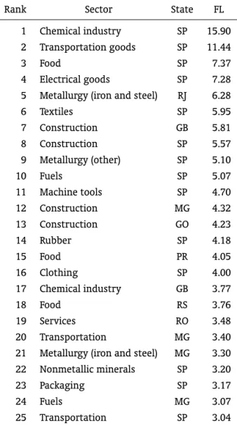
We calculated forward linkages in this fashion for each sector within each state relative to the national economy. The 25 largest linkages are presented in Table 1.
Table 1: Largest Forward Linkages
Rank Sector State FL
1 Chemical industry SP 15.90
2 Transportation goods SP 11.44
3 Food SP 7.37
4 Electrical goods SP 7.28
5 Metallurgy (iron and steel) RJ 6.28
6 Textiles SP 5.95
7 Construction GB 5.81
8 Construction SP 5.57
9 Metallurgy (other) SP 5.10
10 Fuels SP 5.07
11 Machine tools SP 4.70
12 Construction MG 4.32
13 Construction GO 4.23
14 Rubber SP 4.18
15 Food PR 4.05
16 Clothing SP 4.00
17 Chemical industry GB 3.77
18 Food RS 3.76
19 Services RO 3.48
20 Transportation MG 3.40
21 Metallurgy (iron and steel) MG 3.30
22 Nonmetallic minerals SP 3.20
23 Packaging SP 3.17
24 Fuels MG 3.07
25 Transportation SP 3.04
The results obtained point at the importance of the state of São Paulo (SP) and of basic industries sectors, such as chemical industry, transportation goods, electrical goods, and metallurgy. However, some traditional industries, such as food or textiles (in SP), also appear as important sectors, having highly ranked forward linkages. Also, the construction sectors of four states (Guanabara – GB, São Paulo – SP, Minas Gerais – MG, Goiás – GO) appear among the largest linkages. SP counted 14 of its 33 sectors within the first 25 largest forward linkages, 18 among the first 50, and 20 among the first 100. The corresponding figures are, respectively: 1, 3, and 4 for Rio de Janeiro (RJ); 2, 5, and 11 for Guanabara (GB); 4, 6, and 6 for Minas Gerais (MG); 1, 3, and 6 for Rio Grande do Sul (RS); and 1, 4, and 6 for Paraná (PR). It is interesting to note that the metallurgical (iron and steel) sector figures twice among the largest 25, in the states of RJ and MG, but not in the state of SP (which ranks 27th). Furthermore, that
the forward linkages presented a much-skewed distribution deserves mention; that is, a few sectors clearly stand out relative to all others. This can already be perceived in Table 1, if we remember that the average of the linkages obtained is 1 (by definition) and that the full list comprises a total of 825 sectors.
Cumulative backward Rasmussen-Hirschman linkages were also calculated for each sector within each state relative to the national economy in traditional fashion, as the column average of the Leontief inverse relative to the average element of that matrix, that is, as:
e′(I−A)−1/(N.R)
/ e′(I−A)−1e/(N.R)2
Some aspects of the results thus obtained draw the attention. First, regardless of the state, there is a clear prevalence of the sectors of wastes, fuels, and packaging among the largest backward linkages. These sectors account for 24 of the 25 largest backward linkages, and 49 of the largest 50. These three sectors come from the original national matrix estimated by Rijckeghem (1967), who called these sec-tors “fictitious,” as previously mentioned, because they have no value added assigned for them. The relatively very high backward linkages obtained for these sectors doubtless stem from this characteris-tic. This is, therefore, a caveat carried over from the original national matrix.
The second important aspect to be noted in the results of the backward linkages is that, disregarding the fictitious sectors, it is the small states of the economy, rather than the large ones, that exhibit the largest linkages — in several cases, in sectors that are usually characteristic of the large states; for example, paper in Mato Grosso (1st), Sergipe (4th), Espírito Santo (5th), Paraíba (5th), and Ceará (9th);
transportation goods in Ceará (10th), Piauí (11th), and Paraíba (13th); electrical goods in Goiás (7th) and
Espírito Santo (21st); or the chemical industry in Piauí (8th).
A third relevant aspect is that some sectors display low variability in the backward linkage along the states, particularly the nonindustrial ones. Indeed, their distribution is, in general, much more homogeneous than that of the forward linkages. All backward linkages are within the range of 0.52 to 1.73, without the presence of clear outliers.
Although we can understand the results obtained, they are certainly to be considered an important caveat of the estimation procedures adopted. For this reason, in the case of backward linkages, we recommend the use of pure backward linkages, as presented below, which take into consideration the economic size of the respective sector in evaluating its relevance, thus reducing the problems discussed here.
Indeed, it is relevant to mention that not even the forward linkages presented above are detached from this issue, as shown by the fact that the sector of services in Rondônia (RO) has the 19thhighest
forward linkage in the economy. But they seem to have been less affected.
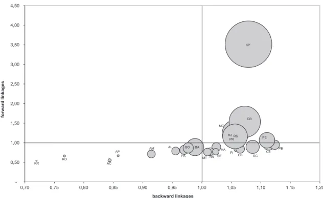
Another perspective of the matrix’s structure can be seized from less disaggregated backward and forward linkages for whole states and whole sectors. We calculated these linkages by means of defini-tions analogous to the ones stated above. We present plots of backward vs. forward linkages in each case in order to grasp the relevance of each state or sector through the consideration of both indicators simultaneously.
Figure 1: Backward vs. Forward Linkages of States
Note: The size of the bubbles represents the states’ GDP.Source: Elaborated by the authors.
character of the regional concentration of the economic structure of the country, as well as a large degree of intra-regional, and even intrastate, endogeneity of intermediate consumption.11
It is interesting to remember that 1959 was precisely the year that theSuperintendência do Desen-volvimento do Nordeste(Superintendence for the Development of the Northeast, SUDENE) was created by the Brazilian government in order to promote the north-eastern region’s development, directing re-sources to that region. The results here obtained point to ashort-termtrade-off between efforts toward regional economic homogenization and national output growth.
Still another perspective to this issue can be reached by looking at Table 2, where we present (type I) output multipliers for each state, splitting the effects that take place inside the state from the ones that take place outside it. Total output multiplier was defined as the average of the column sums for every sector within each state, that is, as e′(I−A)−1eR
/N whereeRis a(N.R×1)state-specific
summation vector with ones in the lines corresponding to state R and zeros in the remaining lines. The inside output multiplier was correspondingly defined as e′
R(I−A)−1eR/N, and the outside output
multiplier as the difference between both.
Once again, we wish to call attention to the larger states. As a rule, these states present an above-average total output multiplier — as expected, because the total output multiplier is related to the backward linkage, presented above. But, more interestingly, the seven states exhibiting a larger pro-portion of inside output multiplier relative to the total output multiplier (RJ, SP, RS, MG, BA, PE, and PR) belong to the eight economically larger states in the country, in which at least 84.5% of the output multiplying effects take place within the state itself. An exception, in this case, is the Federal District (GB), the 16th on the list, with inside output multiplier of 78.7%. Note that these results depict that the relevant economic division is not so much the one between small and large states but rather the one between each of the large states. This is because the large states present larger inside output mul-tipliers; that is, the effects of a variation in demand in any of these states unfold morewithineach one of them, than is the case for the smaller states. Of course, this reasoning is only relative. In order to decide whether, for example, an inside output multiplier larger than 88% (as in the case of SP and RJ) is “high” in a more absolute sense, we would have to provide for relevant points of comparison, which we are unable to supply within our current framework.
While the focus of this paper is the regional dimension of the Brazilian economic structure, this being the new characteristic of the matrix we are using for our analysis, before we move on to pure linkages, in Figure 2 we briefly present Rasmussen-Hirschman backward and forward linkages for whole sectors because, although the original national matrix can produce a similar set of results, the linkages obtained for whole states from the interstate matrix are expectedly different.
Denominating key sectors as the ones that have both above-average backward and forward link-ages, we find in this group the sectors of fuels, packaging, construction, food, transportation, chemical industry, metallurgy of iron and steel, and transportation goods. Once again, we find the fictitious sectors to have very high backward linkages, for the same reasons discussed above.
Pure linkages can provide still another perspective to the structure of the estimated interstate input-output matrix by emphasizing the value of input-output in identifying key sectors and regions, complement-ing the outlook rendered by the cumulative Rasmussen-Hirschman linkages presented and discussed above.
The computation of pure linkages12is based on a partition of the matrix of technical input
coeffi-cients,A:
A= "
Ajj Ajr
Arj Arr
#
11A similar polarized pattern of regional inequalities operating through structural interdependence among regions was found in
Colombia in a recent study by Perobelli et al. (2010).
Table 2: Total, Inside, and Outside Output Multipliers for States
Region State Output Multipliers
Total Inside Outside
North
RO 1.47 1.15 (78%) 0.32 (22%)
AC 1.61 1.22 (76%) 0.39 (24%)
AM 1.75 1.46 (84%) 0.29 (16%)
RR 1.38 1.13 (82%) 0.25 (18%)
PA 1.86 1.40 (75%) 0.46 (25%)
AP 1.64 1.23 (75%) 0.41 (25%)
Northeast
MA 1.96 1.54 (79%) 0.42 (21%)
PI 2.03 1.63 (80%) 0.40 (20%)
CE 2.13 1.75 (82%) 0.38 (18%)
RN 1.94 1.57 (81%) 0.37 (19%)
PB 2.15 1.67 (78%) 0.48 (22%)
PE 2.13 1.80 (85%) 0.33 (15%)
AL 1.83 1.42 (78%) 0.41 (22%)
East
SE 1.96 1.52 (77%) 0.44 (23%)
BA 1.89 1.61 (85%) 0.29 (15%)
MG 2.02 1.75 (87%) 0.27 (13%)
ES 2.04 1.60 (79%) 0.43 (21%)
RJ 2.02 1.79 (89%) 0.22 (11%)
GB 2.05 1.62 (79%) 0.44 (21%)
South
SP 2.07 1.83 (89%) 0.23 (11%)
PR 2.02 1.71 (85%) 0.31 (15%)
SC 2.08 1.73 (83%) 0.35 (17%)
RS 2.02 1.76 (87%) 0.26 (13%)
Center-west MT 1.93 1.56 (81%) 0.37 (19%)
GO 1.87 1.43 (76%) 0.44 (24%)
Notes: The regional grouping follows the 1959 census. The percent-ages indicated are the shares of the total output multiplier for each state.
Figure 2: Backward vs. Forward Linkages of Sectors
Note: The size of the bubbles represents the sectors’ total output. Source: Elaborated by the authors.
wherejdenotes a sector, or a group of sectors, of interest — in our case, a sector within a state — and rthe remaining sectors of the matrix. Pure backward linkages (PBL) and pure forward linkages (PFL) were calculated as:
PBL=e∆rArj∆jYj
PFL=∆jAjr∆rYr
where a)∆r≡(I−Arr)−1, b)∆j≡(I−Ajj)−1, c)Yjis the total output of sector(s)j; and d)Yris
a((N.R−1)×1)vector with the respective total outputs of the remaining sectors. Pure total linkages (PTL) were defined as the sum of PBL and PFL.
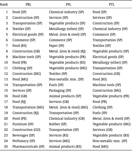
Table 3 presents the ranking of the 25 largest linkages for each of the three indicators.
As expected, given the characteristic of pure linkages and the results presented above, the econom-ically larger states appear in prominence. Moreover, São Paulo clearly stands out even among the large states. It has 14 of the 25 largest PBL, 15 of the 25 largest PFL, and 16 of the 25 largest PTL.
Table 3: Largest Backward, Forward, and Total Pure Linkages
Rank PBL PFL PTL
1 Food (SP) Chemical industry (SP) Food (SP)
2 Construction (SP) Services (SP) Services (SP)
3 Transportation (SP) Vegetable products (SP) Construction (SP)
4 Textiles (SP) Metallurgy (other) (SP) Chemical industry (SP)
5 Electrical goods (SP) Metal. (iron & steel) (SP) Commerce (SP)
6 Commerce (SP) Commerce (SP) Transportation (SP)
7 Food (RS) Paper (SP) Textiles (SP)
8 Construction (GB) Metal. (iron & steel) (RJ) Vegetable products (SP)
9 Machine tools (SP) Vegetable products (PR) Electrical goods (SP)
10 Food (PR) Vegetable products (RS) Metallurgy (other) (SP)
11 Clothing (SP) Vegetable products (MG) Transportation (SP)
12 Construction (MG) Textiles (SP) Construction (GB)
13 Food (MG) Non-metallic min. (SP) Food (RS)
14 Transportation (SP) Fuels (SP) Machine tools (SP)
15 Services (SP) Packaging (SP) Construction (MG)
16 Food (GB) Animal products (SP) Vegetable products (PR)
17 Food (RJ) Services (GB) Food (PR)
18 Transportation (MG) Metal. (iron & steel) (MG) Clothing (SP)
19 Construction (RJ) Transportation (SP) Fuels (SP)
20 Food (PE) Chemical industry (GB) Metal. (iron & steel) (SP)
21 Furniture (SP) Rubber (SP) Vegetable products (MG)
22 Construction (GO) Transportation (SP) Services (GB)
23 Beverages (SP) Services (RS) Vegetable products (RS)
24 Perfumery (SP) Services (MG) Non-metallic min. (SP)
25 Pharmaceuticals (SP) Animal products (RS) Food (MG)
services (GB, RS, and MG), and chemical industry (GB). This isper senot a statement about the diversi-fication of each of these states’ economy. Nevertheless, given that these linkages were calculated and ranked according to the respective sectors’ importance relative to the national economy, these results give an interesting assessment not only of the size of the economy of the state of SP within the Brazilian economy, which is a well-known fact, but also of the state’s structural importance.
4. FINAL COMMENTS
This paper has presented an overview of the regional economic structure of Brazil in 1959 through the estimation of an interstate input-output matrix. One of the main contributions of this paper is the estimated matrix, which thus becomes available to other researchers on request to the authors. The matrix here presented is the oldest interstate matrix for Brazil. Hence, it can be an important tool for the study of the regional productive structure at an historical moment in which the regional question appeared as a central national issue. The limitations and caveats of the matrix — stemming from the original national matrix, from limited sources of data, and from the estimation procedures adopted — were pointed out and discussed in the paper and should be kept in mind, though.
We have characterized the matrix from two different perspectives. First, from a methodological point of view, we provided a detailed description of the data sources, estimation procedures, and hy-potheses used. The estimation was made based on Rijckeghem’s (1967) national matrix for 1959 and on additional data obtained from several sources, using simple and cross-industry location quotients.
Second, we also provided a panoramic structural portrait of the estimated matrix, through the use of selected indicators. The distinguished features of the results included the assessment of the structural importance, besides their economic size, of the larger states, particularly of São Paulo, as well as some evidence of economic introversion of each of these large states, when compared to the smaller ones.
BIBLIOGRAPHY
Baer, W., da Fonseca, M. A. R., & Guilhoto, J. J. M. (1987). Structural changes in Brazil’s industrial economy, 1960-80. World Development, 15(2):275–286.
Brasil (1967a). VII Recenseamento Geral do Brasil, Censo agrícola de 1960. Série nacional, Volume II – 1aparte, IBGE – Serviço Nacional de Recenseamento, Rio de Janeiro.
Brasil (1967b). VII Recenseamento Geral do Brasil, Censo industrial de 1960. Série nacional, Volume III, IBGE – Serviço Nacional de Recenseamento, Rio de Janeiro.
Brasil (1967c). VII Recenseamento Geral do Brasil, Censos comercial e dos serviços de 1960. Série nacional, Volume IV, IBGE – Serviço Nacional de Recenseamento, Rio de Janeiro.
Brasil (1968). VII Recenseamento Geral do Brasil, Censo industrial de 1960: Matérias-primas e produtos. Série especial, Volume V, Fundação IBGE – Instituto Brasileiro de Estatística, Serviço Nacional de Recenseamento, Rio de Janeiro.
Brasil (n.d.). VII Recenseamento Geral do Brasil, Censo demográfico de 1960. Série nacional, Volume I, Fundação Instituto Brasileiro de Geografia e Estatística, Departamento de Estatísticas da População, [Rio de Janeiro].
Cai, J. & Leung, P. (2004). Linkage measures: A revisit and suggested alternative. Economic Systems Research, 16(1):65–85.
Escobedo, F. & Oosterhaven, J. (2008). Hybrid interregional input-output construction methods. Phase one: Estimation of RPCs. Paper presented on the International Input-Output Meeting on Managing the Environment, Seville, Spain, July 9-1.
Fundação Getulio Vargas (1961). Contas nacionais. Revista Brasileira de Economia, 15(1).
Guilhoto, J. J. M., Sonis, M., & Hewings, G. J. D. (2005). Linkages and multipliers in a multiregional framework: Integration of alternative approaches. Australasian Journal of Regional Studies, 11(1):75– 89.
Guilhoto, J. J. M., Sonis, M., Hewings, G. J. D., & Martins, E. B. (1994). Índices de ligações e setores chave na economia brasileira: 1959-1980. Pesquisa e Planejamento Econômico, 24(2):287–314.
IBGE (1961). Anuário estatístico do Brasil – 1961. Ano XXII, IBGE – Conselho Nacional de Estatística, Rio de Janeiro.
IBGE (1963). Classificação de indústrias: Produtos – Matérias-primas. IBGE - Instituto Brasileiro de Geografia e Estatística, Serviço Nacional de Recenseamento. Rio de Janeiro.
Ichihara, S. M. (2007). O uso combinado de modelos insumo-produto e técnicas de geoprocessamento. Tese de doutorado em Economia Aplicada, ESALQ-USP, Piracicaba.
James, J. A. (1984). The use of general equilibrium analysis in economic history.Explorations in Economic History, 21(3):231–253.
Jones, M. E. F. (1985). Regional employment multipliers, regional policy, and structural change in inter-war Britain. Explorations in Economic History, 22(4):417–439.
Miller, R. E. & Blair, P. D. (1985). Input-Output analysis: Foundations and extensions. Prentice-Hall, New Jersey.
Oosterhaven, J. (2005). Spatial interpolation and disaggregation of multipliers. Geographical Analysis, 37(1):69–84.
Oosterhaven, J., Eding, G. J., & Stelder, D. (1999). Clusters, forward and backward linkages, and bi-regional spillovers: Policy implications for the two Dutch mainport regions and the rural north. Paper presented at the 39thEuropean Congress of the Regional Science Association International, August
23-27, University College Dublin.
Oosterhaven, J. & Stelder, D. (2007). Regional and interregional IO analysis. Faculty of Economics and Business, University of Groningen, mimeo.
Perobelli, F. S., Haddad, E. A., Moron, J. B., & Hewings, G. J. D. (2010). Structural interdependence among Colombian departments. Economic Systems Research, 22(3):279–300.
Rijckeghem, W. v. (1967). Tabela de insumo-produto, Brasil – 1959. Texto para discussão do IPEA. With the collaboration of Sérgio Alípio de Oliveira Camargo.
Rijckeghem, W. v. (1969). An intersectoral consistency model for economic planning in Brazil. In: Ellis, Howard S. (Ed.).The economy of Brazil. Berkeley and Los Angeles, University of California Press. pp. 376–401.
Sonis, M., Guilhoto, J. J. M., Hewings, G. J. D., & Martins, E. B. (1995). Linkages, key sectors and structural change: Some new perspectives. The Developing Economies, XXXII(3):233–270.
5. APPENDIX
This appendix describes in some detail the sources of data and the hypotheses assumed for the compilation of the eight matrices, in the form Sector by State, of additional (regional) information used to estimate the interstate input-output table from Rijckeghem’s national table. The eight matrices comprise information on: a) the distribution by state of the (origin of) production of each sector (1); b) the distribution by state of the (origin of) value added, including gross returns to capital (2) and wages, salaries, and social security (3); and c) the distribution by state of the (destination of) final demand, including household consumption (4), government consumption (5), investment (6), exports (7), and imports (8).
• Origin of production by state: Information on the 33 productive sectors came respectively from:
– Sectors 1 and 2, agricultural sectors: The data source used was the national accounts (Fun-dação Getulio Vargas, 1961, pp. 92–5), which was the same source Rijckeghem used in his estimates. It was necessary to estimate production for the states of RO, AC, RR, and AP, as this information was not reported in the national accounts. The estimation was done pro-portionately to the agricultural workforce in 1959 (pessoal ocupado na agricultura) relative to that in the other states of the northern region, as obtained from the Agricultural Census (Brasil, 1967a, p. 26).
– Sector 3, electric energy: The production of electric energy by state was estimated from the data on electric energy consumption that we found; hence, there is an implicit hypothesis here regarding the non-tradability of this product between states. Data on industrial con-sumption of electric energy (39% of total electric energy production) by state were found in the Industrial Census (Brasil, 1967b, p. 119). The remainder of the value in the national table was then distributed proportionately to the consumption of electric energy in the municipalities of the states’ capitals in 1959 (IBGE, 1961, p. 276).
– Sectors 4 and 5, commerce and services: Commerce by state was estimated proportionally to the commercial flux (giro comercial) in 1959; data found in the Statistical Yearbook (IBGE, 1961, p. 263), which was in turn calculated from data on sales tax’s (imposto sobre vendas e consignações) collection. Services by state were also supposed to be non-tradable and were estimated from primary data or estimates of expenditures on services by state of each sector. Data on industrial expenditure on services (17% of total services) were obtained from the Industrial Census (Brasil, 1967b, pp. 119–20), while data on commercial expendi-ture on services (13%) were obtained from the Commerce and Service Census (Brasil, 1967c, p. 67). The expenditures on commerce of the primary, electric energy, transportation, and construction sectors (adding up to 6%) were estimated proportionately to their respective production by state. Household expenditure on commerce (60%) was estimated proportion-ately to each state’s internal income in 1959 (IBGE, 1961, p. 269). Finally, the service sector self-consumption (4%) was estimated proportionately to the service expenditure by state of the remaining sectors.
production) by state was obtained from the Industrial Census (Brasil, 1967b, p. 119). The ex-penditure on fuels of the primary, electric energy, commerce, services, transportation, and construction sectors (adding up to 56%) was estimated proportionately to their respective production by state. Government fuel consumption (4%) was estimated proportionately to public employees by state (Brasil, nd, p. 101). Household fuel consumption (11%) was estimated proportionately to each state’s internal income in 1959 (IBGE, 1961, p. 269). Ex-port fuel consumption (0.1%) was assumed to be proEx-portional to the exEx-ported tonnage in 1959 (IBGE, 1961, p. 220). Data on the industrial expenditure on packaging (92% of total packaging production) were obtained from the Industrial Census (Brasil, 1967b, p. 119). The packaging expenditure of the vegetable products sector (8%) was estimated proportionally to its production by state.
– Sectors 9 to 31, industrial sectors: The data on the production by state of the industrial sectors were the best we were able to obtain, and this is crucial given the importance of these sectors for several purposes in input-output analyses. Indeed, the information is not only fully compatible with the one used by Rijckeghem for the national matrix but also his and ours best-quality data. These were found in the Industrial Census (Brasil, 1967b, pp. 92-114).
∗ Sectors 11 and 12, metallurgical sectors: Data on the disaggregated metallurgical sec-tors by state were not readily available from the National Series of the Industrial Cen-sus. In order to reconstruct them, we used two special publications of the Industrial Census. A detailed classification of industries, which served as the norm for the tabular presentation of the results of the Industrial Census of 1960 (IBGE, 1963), allowed us to produce a list of products for the “metallurgical (iron and steel)” sector that was con-sistent with the original aggregated data, which included “Steel products – iron and steel”, “Steel products – alloys”, and part of “Various metallurgical products”. The pro-duction by state of each product on this list was then found in the Special Series of the Industrial Census (Brasil, 1968). The “metallurgical (other)” sector was then calculated as the residual from the aggregated metallurgical sector (Brasil, 1967b, p. 95).
– Sectors 32 and 33, construction and transportation: The construction sector production by state was estimated as proportional to the consumption of cement in 1959 (IBGE, 1961, pp. 277–78). The transportation sector production was estimated from information or es-timates on transportation expenditure by state for several sectors. The expenditures on transportation of the industrial and commercial sectors (adding up to 17% of total trans-portation) were found in their respective censuses (Brasil, 1967b, p. 120; Brasil, 1967c, p. 67). Household expenditure on transportation (54%) by state was assumed to be proportional to the total population of each state (Brasil, nd, p. 80). The expenditures on transportation of the Construction and Services sectors (adding up to 3%) were assumed to be proportional to their respective production. The export sector expenditure on transportation (8%) was assumed to be proportional to the exported tonnage in 1959 (IBGE, 1961, p. 220). Govern-ment expenditure on transportation (16%) was assumed to consist of subsidies and hence was distributed by state proportionately to the sum of the above-mentioned transport ex-penditures. Transportation self-consumption (2%) was assumed to be proportional to the remaining sectors’ expenditures on transportation.
and social security in the industrial sectors add up to 25% of the total WSSS. Data on the wages, salaries, and social security paid by the commercial sector (8%) was obtained from the Commerce Census (Brasil, 1967c, pp. 64, 67). The wages, salaries, and social security paid by the government (16%) were assumed to be proportional to the number of public employees by state (Brasil, nd, p. 101), and those paid by households (7%) were assumed to be proportional to the internal income by state (IBGE, 1961, p. 269). The wages, salaries, and social security from the remaining sectors (adding up to 44%) were assumed to be proportional to their respective production by state. To estimate the gross returns to capital of the industrial sectors (adding up to 30% of the total GRC), we initially estimated the value added by state (but aggregated for sectors) from data obtained from the Industrial Census (Brasil, 1967b, pp. 119–20). This was then distributed among sectors within each state proportionately to the value of industrial transformation found in the Industrial Census (Brasil, 1967b, pp. 92–114). This resulted in an estimate for the value added by sector and by state. The gross returns to capital of the industrial sectors were finally obtained by subtracting from the value added the respective wages, salaries, and social security that we had already estimated. The gross returns to capital of the remaining sectors (70%) were assumed to be proportional to their respective production by state.