, v.60, n.1, p.97-103, Jan./Mar. 2003
VARIANCE ADDITIVITY OF GENETIC POPULATIONAL
PARAMETER ESTIMATES OBTAINED
THROUGH BOOTSTRAPPING
Luciana Aparecida Carlini-Garcia1; Roland Vencovsky1*; Alexandre Siqueira Guedes Coelho2
1
Depto. de Genética - USP/ESALQ, C.P. 83 - CEP: 13418-970 - Piracicaba, SP. 2
Depto. de Biologia Geral - UFG/ICB, C.P. 131 - CEP: 74001-970 - Goiânia, GO. *Corresponding author <rvencovs@esalq.usp.br>
ABSTRACT: Studying the genetic structure of natural populations is very important for conservation and use of the genetic variability available in nature. This research is related to genetic population structure analysis using real and simulated molecular data. To obtain variance estimates of pertinent parameters, the bootstrap resampling procedure was applied over different sampling units, namely: individuals within populations (I), populations (P), and individuals and populations simultaneously (I, P). The considered parameters were: the total fixation index (F or FIT), the fixation index within populations (f or FIS) and the divergence among populations or intrapopulation coancestry (θ or FST). The aim of this research was to verify if the variance estimates of Fˆ, fˆ and θˆ, found through the resampling over individuals and populations simultaneously (I, P), correspond to the sum of the respective variance estimates obtained from separated resampling over individuals and populations (I+P). This equivalence was verified in all cases, showing that the total variance estimate of Fˆ, fˆ and θˆ can be obtained summing up the variances estimated for each source of variation separately. Results
also showed that this facilitates the use of the bootstrap method on data with hierarchical structure and opens the possibility of obtaining the relative contribution of each source of variation to the total variation of estimated parameters.
Key words: population structure, resampling, molecular markers, natural populations, simulation
ADITIVIDADE DE VARIÂNCIAS OBTIDAS POR BOOTSTRAP DE
ESTIMATIVAS DE PARÂMETROS GENÉTICOS POPULACIONAIS
RESUMO: O estudo da estrutura genética de populações naturais é muito importante para a conservação e o uso da variabilidade genética disponível na natureza. Esta pesquisa relaciona-se com a análise da estrutura genética de populações a partir de dados moleculares reais e simulados. Visando estimar variâncias de estimativas de parâmetros pertinentes, o método de reamostragem bootstrap foi aplicado levando em conta diferentes unidades amostrais, a saber: indivíduos dentro de populações (I), populações (P) e indivíduos e populações concomitantemente (I, P). Os parâmetros considerados foram: o índice de fixação total (F ou FIT), o indice de fixação intrapopulacional (f ou FIS) e a divergência interpopulacional (θ ou FST). O trabalho objetivou estimar a variância amostral das estimativas destes parâmetros para verificar se as variâncias de Fˆ, fˆ e θˆ, obtidas pela reamostragem de indivíduos e populações concomitantemente (I, P) são equivalentes às obtidas pela soma (I+P) das variâncias estimadas reamostrando-se I e P separadamente. A equivalência foi verificada em todos os casos investigados, mostrando ser possível estimar as variâncias das estimativas de Fˆ, fˆ e θˆ para cada fonte de variação (unidade amostral) somando-as depois para estimar a variância total. O procedimento facilita o uso do método bootstrap em dados com estrutura hierárquica e permite mensurar a importância relativa de cada fonte de variação sobre a variância amostral total das estimativas dos parâmetros. Palavras-chave: estrutura populacional, reamostragem, marcadores moleculares, populações naturais, simulação
INTRODUCTION
In studies of genetic population structure with the use of genetic markers, usually resampling methods are used to estimate genetic population parameters and their respective standard deviation. Some authors have used resampling only over one source of variation, like Van Dongen (1995) and Vencovsky et al. (1997), who applied it only over individuals. Others applied it over several sources of variation, such as Petit & Pons (1998) and Carlini-Garcia et al. (2001).
Petit & Pons (1998) applied the bootstrap method over individuals, populations, and individuals and
populations concomitantly, to estimate population parameters and their variances, based on these sources of variation. Their objective was to verify over which source of variation resampling should be applied to obtain estimates of the studied parameters. To do so, they compared the obtained variances based on the mentioned variation sources, with the variance estimates calculated from explicit expressions obtained by Pons & Petit (1995). The authors concluded that to estimate the studied parameters and their variances, the resampling should be priority over populations.
, v.60, n.1, p.97-103, Jan./Mar. 2003
population, populations and individuals simultaneously, and also over loci. They estimated some genetic population parameters, their standard deviation, and obtained the respective confidence intervals, as well as the empirical distribution of the estimates. Among other aspects, they could demonstrate the importance of applying resampling taking into account each source of variation.
The aim of this research was to verify if, with the hierarchically structured data, it is possible to obtain the total bootstrap variance of an estimate summing up all obtained variances by the resampling over each source of variation separately. This equivalence would be advantageous in that it would be possible to obtain the relative contribution of population and individual sources of variation to the total variation, as well as the lack of necessity to do a joint resampling of individuals and populations. The hierarchical structure considered involved populations and individuals within populations. The evaluated parameters were the total fixation index
(F or FIT), the fixation index within populations (f or FIS)
and the degree of divergence among populations or
coancestry within populations (θ or FST) (Wright, 1951;
1965; Cockerham, 1969; 1973; Weir & Cockerham, 1984; Weir, 1996). Real and simulated data were considered.
MATERIAL AND METHODS
The data used in this research were obtained by Telles & Coelho (1998), Ciampi (1999), Auler (2000), Reis et al. (2000), Seoane et al. (2000) and Sebbenn et al. (2001). These authors studied the population genetic structure and/or reproductive system of tropical arboreous trees, by means of isoenzymatic markers or, in the case of Ciampi (1999), by microsatelite markers.
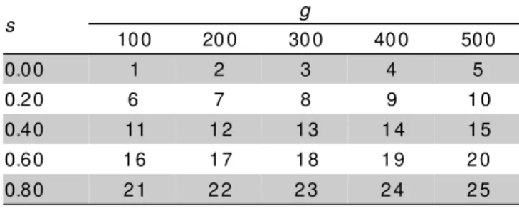
Twenty-five sets of simulated data were also used, each of them composed by 30 populations with 100 individuals each. Five loci with three alleles per locus were considered, and the initial allelic frequencies were 1/3 for each allele at all loci. In these simulations, populations in inbreeding equilibrium were considered
with the inbreeding rates (s) varying in the interval 0 ≤s
≤ 0.08 and the number of generations (g) varying from
100 to 500 (Table 1). Different numbers of generations were considered to generate data sets having different degrees of divergence among populations.
The study of population genetic structure of each considered data set was carried out by means of analysis of variance of gene frequencies (Cockerham, 1969; 1973; Weir & Cockerham, 1984; Weir, 1996). Thus, in each
case, the total variance estimate ( 2
T
σˆ ) of the allelic
frequencies, as well as their components: among
populations ( 2
P
σˆ ), among individuals within populations
( 2
I
σˆ ), and among genes within individuals (σˆG2), were
obtained. From these, estimates of the total fixation index
(Fˆ), the fixation index within populations (fˆ), and the
degree of divergence among populations or coancestry
within populations (θˆ) and their respective variance
estimates, were calculated.
To obtain these estimates, a random model was considered, meaning that for each data set, it was assumed that there is a reference population that originated, by genetic drift, the evaluated populations. Therefore no selection in all considered loci was assumed, such that loci were taken as neutral. The considered hierarchical structure for the analysis of variance included the following sources of variation: populations (P), individuals within populations (I) and genes within individuals (G) (Weir, 1996).
The method of moments was employed to estimate the variance components mentioned above, as well as to estimate the other population parameters, according to Weir (1996):
2 2 2 2 2 G I P I P ˆ ˆ ˆ ˆ ˆ Fˆ σ σ σ σ σ + + + = 2 2 2 2 G I P P ˆ ˆ ˆ ˆ ˆ σ σ σ σ θ + + = θ θ ˆ ˆ Fˆ fˆ − − = 1
The resampling bootstrap method (Efron & Tibshirani, 1993; Manly, 1997) was applied with the
objective of obtaining bootstrap estimates of F, f and θ
and of their respective variance estimates, considering the sources of variations of individuals, populations, and individuals and populations simultaneously, in a similar way to that used by Petit & Pons (1998), fixing the loci. In each resampling level, 100,000 bootstrap samples were obtained for the real data and 10,000 for the simulated data. The variance analysis was carried out in
each bootstrap sample, which provided F, f and θ
estimates. The average of these estimates, per parameter, is the bootstrap estimate of the parameter, while their variance is the variance estimate of the bootstrap estimate of the parameter.
For F, f and θ parameters individually, it was
verified if the additivity of the variances was true or not when the bootstrap approach is used. This property was investigated verifying if the sum of the variance estimates of the parameter estimates, obtained from the independent resampling of individuals and populations, corresponds to the variance estimate of such parameter estimates, taken from the concomitant resampling of individuals and populations. In addition to the practical
s g
10 0 20 0 30 0 40 0 50 0
0.00 1 2 3 4 5
0.20 6 7 8 9 1 0
0.40 11 1 2 1 3 1 4 1 5
0.60 1 6 1 7 1 8 1 9 2 0
0.80 2 1 2 2 2 3 2 4 2 5
, v.60, n.1, p.97-103, Jan./Mar. 2003
facility of not having to carry out the simultaneous resampling of populations and individuals, the outlined procedure allows investigating the relative contribution of the sources of variation and gives an indication of where the major deficiencies of field sampling are occurring.
To verify this additivity, a simple linear regression
model was adopted, i.e. Y = α +βX + ε,Y being the values
of the sum the variances obtained from the resampling of
individuals and populations separately, and X the
respective variance estimated from the simultaneous resample of these two factors. This was carried out for
each parameter (F, f and θ),with the simulated and real
data sets. Student’s t tests were applied to verify if the
coefficient of regression (β) and the intercept (α) estimates
differed from zero. Confidence intervals for β were
constructed to verify if the corresponding parameter
differed from 1 (Sokal & Rohlf, 1995). If α = 0, β≠ 0 and β
does not differ from 1, the regression equation is reduced
to E (Y) = X in terms of mathematical expectation, and
then, it is possible to confirm the additivity of variance estimates, that were derived from the resample of individuals and populations separately. The degree of deviations from regression was verified through the
coefficients of determination R2, obtained for each
regression analysis (Sokal & Rohlf, 1995).
Shapiro-Wilk test was applied to verify if the regression analysis residuals follow a normal distribution (Sokal & Rohlf, 1995). When this assumption was not fulfilled, appropriate data transformation was searched for attaining normality. This was necessary to guarantee the validity of the test of hypothesis, as well as the confidence intervals calculated for the intercept and for the coefficient of regression, which are based on normality.
As these two variables involved in the regression are random, an appropriate regression analysis for the random model could have been used (geometric mean regression; Sokal & Rohlf, 1995). Nevertheless, these latter authors mention the existence of controversies regarding the use of this methodology. Thus, the usual regression analysis was used here, as described in the previous paragraphs, in agreement with Neter et al. (1990).
All resamplings and calculations of F, f and θ
bootstrap estimates and of their bootstrap variances estimates were carried out using a version of the EG software (Coelho, 2000), specially developed for this purpose.
RESULTS AND DISCUSSION
For the real data sets, the observed values (total variance estimates, due to individuals and populations together: I, P) and the expected values of these variances (sum of estimates of variances due to the sources of variation of individuals and populations, I+P) were very close (Table 2). In the case of Seoane’s et al. (2000) data, the bootstrap discard did not contribute in a significant manner to the increase in the difference between the
estimates, as the discard was very small, from 0.011% and 0.014%, for individuals, and individuals and populations simultaneous resamples, respectively. However, these discards must have altered the precision of the estimates and of their variances, in comparison to those obtained with no discards. These discards are due to the estimation method used, since estimates were obtained as variance ratios and, in certain combinations, these ratios may have zero values in the denominators. In these cases, the software used automatically discarded the bootstrap sample. This procedure was applied to all resampling levels.
Shapiro-Wilk’s normality test was non-significant
(P ≥ 0.05) in all analyses, when the real data set was
considered. This, however, was not observed with the
simulated data in the case of the F and θ.
Nevertheless, the regression residuals presented normal distribution when the logarithmic transformation was applied to the simulated data sets for these two parameters.
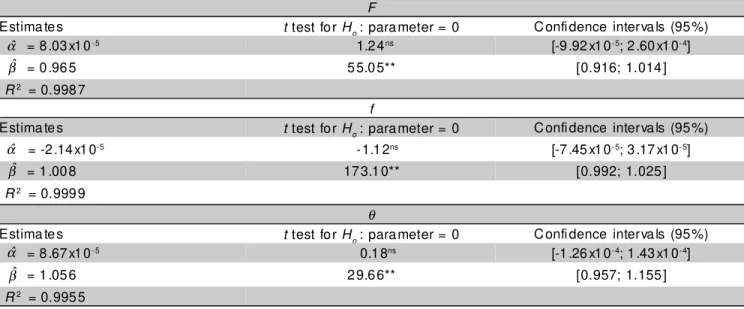
In all situations, the linear regression model adjusted well to the data. In all the real cases, the
estimates of β were significant, and intercept estimates (αˆ)
did not differ from zero. Furthermore, in all regressions,
the hypothesis β = 1 was accepted since all confidence
intervals obtained for β included the value 1. Deviations
from regression were not expressive, since all R2 values
were greater than 99% (Table 3, Figure 1 i to iii).
Results obtained for the three parameters indicated that the corresponding variance estimates, taken from individual and population resamples, can be summed up to obtain the total variance due to these two sources of variation jointly, confirming the additivity of the
variances. Therefore, the regression model reduces to Y
= X + ε. This same behavior was also observed when
the simulated data sets were analyzed. In this case, the observed and expected values of the total variance
estimates of Fˆ, fˆ and θˆ were even more similar (Table
4). Such an outcome is probably due to the large number of populations and individuals used in each data set. No bootstrap discards took place.
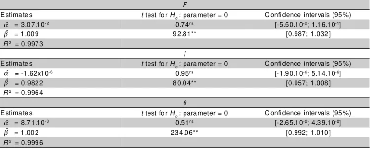
Results of the simulated data confirmed those obtained with the real data. In all cases the null
hypotheses H0 : α and H0 : β = 1 were not rejected. All
the R2 values were greater than 99%, so that deviations
, v.60, n.1, p.97-103, Jan./Mar. 2003
and populations simultaneously, the concomitant resampling of these two sources of variation becomes
necessary whenever the distribution of the estimates Fˆ,
fˆ and θˆ is unknown. However, in order to investigate if
the parameter differs or not from zero, an alternative approach is analyzing jointly the confidence intervals obtained for each resampled level. Carlini-Garcia et al.
a, bintercept and coefficient of regression, respectively; c, d, e estimates of the total fixation index, the fixation index within populations, and the divergence among populations, respectively; ns non-significative; **(P ≤ 0.01).
Table 3 - aα and bβ estimates and respective confidence intervals for the regression of observed (I, P) and expected (I+P)
values of the cFˆ, dfˆ and eθˆ variance estimates. Estimates of the coefficient of determination R2. Data from
several authors.
(2001) proposed that, if at least one of the confidence intervals, for a given parameter, comprised the zero value, the parameter should be considered null. Under this criterion, the hypothesis that the parameter is null is rejected only when all confidence intervals do not contain the zero value. The reference value zero is adequate for
F, f and θ , but can be different for other parameters.
F
Estima tes t test for Ho : parameter = 0 C onfidence intervals (95%)
= 8.03x10⁻⁵ 1.24ns [-9.92 x10⁻⁵; 2.60 x10⁻⁴]
= 0.965 55.05** [0.916; 1.014]
R2 = 0.9987
f
Estima tes t test for Ho : parameter = 0 C onfidence intervals (95%)
= -2.14x10⁻⁵ -1.12ns [-7.45 x10⁻⁵; 3.17 x10⁻⁵]
= 1.008 173.1 0** [0.992; 1.025]
R2 = 0.9999
θ
Estima tes t test for Ho : parameter = 0 C onfidence intervals (95%)
= 8.67x10⁻⁵ 0.18ns [-1.26 x10⁻⁴; 1.43 x10⁻⁴]
= 1.056 29.66** [0.957; 1.155]
R2 = 0.9955
Telles & Coelho (1998) Ciampi (1999)
Level dndb Level dndb
I 0 12.55 18.39 3.34 I 0 1.48 1.83 0.29
P 0 35.38 16.62 19.71 P 0 4.25 3.57 1.68
I+P - 47.93 35.01 23.06 I+P - 5.73 5.40 1.97
I, P 0 49.31 35.34 22.81 I, P 0 5.78 5.33 1.86
Auler (2000) Reis et al. (2000)
Level dndb Level dndb
I 0 8.51 8.19 0.80 I 0 5.38 5.98 0.50
P 0 26.36 26.73 0.58 P 0 16.03 13.69 0.37
I+P - 34.87 34.92 1.39 I+P - 21.41 19.67 0.87
I, P 0 34.91 34.78 1.39 I, P 0 21.64 19.74 0.88
Seoane et al.(2000) Sebbenn et al. (2001)
Level dndb Level dndb
I 11 20.99 29.23 5.95 I 0 9.30 6.95 3.40
P 0 35.97 30.56 9.73 P 0 16.36 0.70 18.13
I+P - 56.96 59.79 15.69 I+P - 25.66 7.65 21.53
I, P 14 58.36 59.31 14.19 I, P 0 24.53 7.88 19.45
a, b, c estimates of the total fixation index, the fixation index within populations, and the divergence among populations, respectively; d number of discarded bootstraps; e, f, g Fˆ, fˆ and θˆ variance estimates, respectively, multiplied by 104.
Table 2 - Variance estimates of aFˆ, bfˆ and cθˆ due to resampling over individuals (I), populations (P), and I and P jointly (I, P).
Sums up I and P variances are show as I+P. Data from several authors.
g f
e e g
g e
g e
g e
g
e f
f
f
f
f
) (fˆ Vˆ )
(Fˆ
Vˆ Vˆ(θˆ) Vˆ(Fˆ) Vˆ(fˆ) Vˆ(θˆ)
) (fˆ Vˆ )
(Fˆ
Vˆ Vˆ(θˆ)
) (fˆ Vˆ )
(Fˆ
Vˆ Vˆ(θˆ)
) (fˆ Vˆ )
(Fˆ
Vˆ Vˆ(θˆ) Vˆ(Fˆ) Vˆ(fˆ) Vˆ(θˆ)
αˆ βˆ
βˆ αˆ
, v.60, n.1, p.97-103, Jan./Mar. 2003
As mentioned in methodology, different combinations of selfing rates and numbers of generations of divergence were considered (Table 1). The variances
of θˆ and Fˆ tend to increase with divergence as expected
(Table 4). Even though, the property of additivity was maintained.
Probably the main advantage of this additivity is the possibility of obtaining the relative contribution of the different sources of variation to the total variation. This fact has implications in sample planning, as the source that most contributes to the total variance should receive
greater attention in the elaboration of future sample strategies. By knowing these relative contributions and verifying trends in several similar types of research, it is possible to organize sampling strategies (number of populations and of individuals per population) to minimize the error in the population parameter estimates.
Obtaining expressions of intrapopulation (among individuals) and interpopulation variance components that contribute to the bootstrap variances is an interesting area for future research. This is specially true when individuals and populations are resampled
Figure 1 - Regressions between observed and expected variance estimates of the Fˆ, fˆ and θˆ. Data from various authors (i to iii), and
simulated and transformed data (iv and vi), and simulated and non-transformed data (v).
f
0.000 0.001 0.002 0.003 0.004 0.005 0.006 0.007
0.000 0.001 0.002 0.003 0.004 0.005 0.006 0.007
y = 1.0083*x - 2.14*10 -5
r2 = 0.9999
Theta
-0.0002 0.0000
0.0002 0.0004
0.0006 0.0008
0.0010 0.0012
0.0014 0.0016
0.0018 0.0020
0.0022 0.0024 -0.0002
0.0000 0.0002 0.0004 0.0006 0.0008 0.0010 0.0012 0.0014 0.0016 0.0018 0.0020 0.0022 0.0024 0.0026
p
y = 1.0562*x + 8.67*10 -6
r2 = 0.9955
Theta
-5 -4.8 -4.6 -4.4 -4.2 -4 -3.8 -3.6 -3.4 -3.2 -5
-4.8 -4.6 -4.4 -4.2 -4 -3.8 -3.6 -3.4 -3.2
y = 1.0016*x + 8.71*10-3
r2 = 0.9996 iv)
ii) v)
iii) vi)
F
0.000 0.001 0.002 0.003 0.004 0.005 0.006 0.007
0.000 0.001 0.002 0.003 0.004 0.005 0.006
p
y = 0.9651*x + 8.03*10 -5
r2 = 0.9987
i)
F
-4.1 -4 -3.9 -3.8 -3.7 -3.6 -3.5 -3.4 -3.3 -3.2
-4.1 -4 -3.9 -3.8 -3.7 -3.6 -3.5 -3.4 -3.3 -3.2
p
y = 1.0091*x + 3.07*10-2
r2 = 0.9973
f
0.0000 0.0001 0.0001 0.0001 0.0001 0.0001 0.0002 0.0002 0.0002 0.0002
Ob d l
0.0000 0.0001 0.0001 0.0001 0.0001 0.0001 0.0002 0.0002 0.0002 0.0002
y = 0.9822*x + 1.62*10-6
r2 = 0.9964
--- Expected V
alues
---
---, v.60---, n.1---, p.97-103---, Jan./Mar. 2003
simultaneously. Petit & Pons (1998), considering Nei’s diversity measures with haploid loci, verified that the variance obtained by the simultaneous resampling of individuals and populations contains the total (intra and interpopulation) and the intrapopulation variances, and not only the total variance. This could not be verified in this, because the explicit expressions of the bootstrap variance components of the evaluated parameters have been necessary.
Considering the real data sets, in approximately 78% of the comparisons, the variance estimates due to the source of variation of populations were superior to the estimated variances due to individuals (Table 2). With the simulated data set, this percentage increased to 91% (Table 4). These results seem to confirm what Petit & Pons’s (1998) obtained, i.e., that the variance estimates, when populations were resampled, contain both the intra and interpopulation variance components. This behavior is pertinent, since when populations are resampled,
individuals belonging to these populations are also resampled. This suggests that variances derived from bootstrap should be considered as mean squares and not as variance components associated to the levels under resampling. Therefore, the number of individuals influences the amount with which the variance component, due to individuals, contributes to the variance due to the populations.
Including the source of variation due to loci in this study would require knowing not only the total bootstrap variance, based on the hierarchical resampled levels (populations and individuals), but also the component due to loci. As the source of variation of loci leads to a crossed data structure, the existence of variance components due to interactions between loci and other resampled levels are expected. Therefore, it is not expected that mean squares are additive when loci are resampled together with individuals and populations. Determining the bootstrap variance components based Table 4 - Variance estimates of aFˆ, bfˆ and bθˆ due to resampling over individuals (I), populations (P), and I and P jointly (I, P).
Sums up variances are show as I+P. Simulated data.
a, b, c estimates of the total fixation index, the fixation index within populations, and the divergence among populations, respectively; d number of discarded bootstraps; e, f, g Fˆ, bfˆand cθˆ variance estimates, respectively, multiplied by 105.
d e f
Data sets I P I+P I e P I P I+P I e P I P I+P I e P
1 3.48 5.34 8.82 8.85 3.44 3.96 7.40 7.49 0.33 1.29 1.62 1.64
2 3.54 7.61 11.15 11.14 3.80 3.29 7.09 7.13 0.56 4.83 5.38 5.38
3 3.57 5.47 9.04 9.11 4.00 2.78 6.79 6.76 0.63 4.57 5.20 5.09
4 3.58 18.36 21.95 22.61 4.13 3.51 7.64 7.63 0.76 14.68 15.44 15.78
5 3.65 20.80 24.45 23.11 4.36 4.48 8.84 8.53 0.84 18.91 19.75 18.70
6 4.72 5.11 9.83 10.15 5.13 3.98 9.11 9.44 0.40 1.79 2.20 2.21
7 4.66 7.25 11.92 11.92 5.34 4.95 10.29 10.26 0.64 4.35 4.99 4.98
8 4.42 13.17 17.59 17.75 5.60 6.28 11.89 11.82 0.72 8.98 9.70 9.62
9 4.52 22.20 26.73 26.64 6.15 6.17 12.33 12.33 0.85 23.44 24.29 24.03
10 4.23 42.02 46.25 46.91 6.39 5.74 12.13 12.18 0.96 43.38 44.35 44.48
11 6.10 8.02 14.12 14.38 6.84 7.03 13.86 14.26 0.51 1.22 1.73 1.68
12 5.76 8.88 14.65 14.65 7.16 6.43 13.59 13.31 0.81 7.27 8.08 8.06
13 5.36 12.93 18.30 19.29 7.35 10.67 18.03 18.59 1.01 11.17 12.18 12.59
14 5.58 13.23 18.81 18.97 8.16 7.84 16.00 15.86 0.95 19.17 20.11 19.77
15 4.97 23.98 28.95 28.19 7.72 9.26 16.98 16.97 1.05 28.64 29.69 28.68
16 6.77 8.99 15.75 15.68 7.74 9.24 16.98 17.18 0.66 3.67 4.33 4.30
17 6.23 6.72 12.95 13.16 8.40 5.91 14.30 14.26 1.00 10.50 11.50 11.44
18 5.74 10.24 15.98 16.22 8.52 10.95 19.47 19.63 1.11 9.81 10.92 10.57
19 5.26 15.32 20.59 20.58 8.58 11.45 20.03 19.86 1.20 27.29 28.49 29.04
20 4.67 15.95 20.62 21.39 8.64 7.23 15.87 16.53 1.31 33.59 34.90 34.94
21 5.15 5.92 11.07 11.31 6.33 6.91 13.24 13.62 0.94 3.98 4.91 5.01
22 5.13 6.10 11.22 11.05 7.25 6.27 13.52 13.26 1.30 7.89 9.19 9.11
23 4.30 4.77 9.08 9.29 7.38 4.35 11.72 11.74 1.51 21.83 23.34 23.66
24 3.84 9.50 13.34 13.55 8.00 8.82 16.82 16.95 1.62 37.43 39.05 38.75
25 3.14 7.46 10.60 10.91 7.85 8.77 16.62 16.84 1.62 41.64 43.26 42.01
) (Fˆ
, v.60, n.1, p.97-103, Jan./Mar. 2003
Received January 4, 2002
on the crossed structure due to loci in addition to those due to the hierarchical structure is necessary. This is required for verifying the property of additivity when loci are resampled together with individuals and populations or even with any other possible hierarchical levels.
REFERENCES
AULER, N.M.F. Caracterização da estrutura genética de populações naturais de Araucaria angustifolia (Bert) O. Ktze. no Estado de Santa Catarina. Florianópolis, 2000. 93p. Dissertação (Mestrado) - Universidade Federal de Santa Catarina.
CARLINI-GARCIA, L.A.; VENCOVSKY, R.; COELHO, A.S.G. Método bootstrap aplicado em diferentes níveis de reamostragem na estimação de parâmetros genéticos populacionais. Scientia Agricola, v.58, p.785-793, 2001.
CIAMPI, A.Y. Desenvolvimento e utilização de marcadores microsatélites, AFLP e seqüênciamento de cpDNA, no estudo da estrutura genética e parentesco em populações de copaíba (Copaifera langsdorffii) em matas de galeria no cerrado. Botucatu, 1999. 204p. Tese (Doutorado) – Instituto de Biociências, Universidade Estadual Paulista “Júlio de Mesquita Filho”. COCKERHAM C.C. Variance of gene frequencies. Evolution, v.23, p.72-84,
1969.
COCKERHAM, C.C. Analysis of gene frequencies. Genetics, v.74, p.679-700, 1973.
COELHO, A.S.G. Programa EG: Análise de estrutura genética de populações pelo método da análise de variância (software). Goiânia: Universidade Federal de Goiânia, Instituto de Ciências Biológicas, Departamento de Biologia Geral, 2000.
EFRON, B.; TIBSHIRANI, R.J. An introduction to the bootstrap. New York: Chapman & Hall, 1993. 436p.
MANLY, B.F.J. Randomization, bootstrap and monte carlo methods in biology. 2. ed. London: Chapman & Hall, 1997. 399p.
NETER, J.; WASSERMAN, W.; KUTNER, M.H. Applied linear regression models. 3. ed. Homewood: Irwin,1990. 1181p.
PETIT, R.J.; PONS, O. Bootstrap variance of diversity and differentiation estimators in a subdivided population. Heredity, v.80, p.56-61, 1998.
a, b intercept and coefficient of regression, respectively; c, d, e estimates of the total fixation index, the fixation index within populations, and the divergence among populations, respectively; ns non-significative; ** (P ≤ 0.01).
PONS, O.; PETIT, R.J. Estimation variance and optimal sampling of gene diversity. I. Haploid locus. Theoretical and Applied Genetics, v.90, p.462-470, 1995.
REIS, M.S.; VENCOVSKY, R.; KAGEYAMA, P.Y.; GUIMARÃES, E.; FANTINI, A.C.; NODARI, R.O.; MANTOVANI, A. Variação genética em populações naturais de palmiteiro (Euterpe edulis Martius – Arecaceae) na floresta ombrófila densa. Sellowia, v.49-52, p.131-149, 2000.
SEBBENN, A.M.; SEOANE, C.E.S.; KAGEYAMA, P.Y.; LACERDA, C.M.B. Estrutura genética em populações de Tabebuia cassinoides: implicações para o manejo florestal e a conservação genética. Revista do Instituto Florestal, v.13, p.99-113, 2001.
SEOANE, C.E.S.; KAGEYAMA, P.Y.; SEBBENN, A.M. Efeitos da fragmentação florestal na estrutura genética de populações de Esenbeckia leiocarpa Engl. (guarantã). Scientia Forestalis, n.57, p.123-139, 2000.
SOKAL, R.R.; ROHLF, F.J. Biometry: the principles and practice of statistics in biolofical research. 3.ed. New York: W.H. Freeman, 1995. 887p. TELLES M.P.C.; COELHO, A.S.G. Caracterização genética de populações
naturais de araticum (Anonna crassiflora). Genetic and Molecular Biology, v.21, p.199, 1998. Supplement. /Apresentado ao 44. Congresso Nacional de Genética, Águas de Lindóia, 1998 – Resumo/
VAN DONGEN, S. How should we bootstrap allozyme data? Heredity, v.74, p.445-447, 1995.
VENCOVSKY, R.; DIAS, C.T.S.; DEMÉTRIO, C.G.B.; LEANDRO, R.A.; PIEDADE, S.M.S. Reamostragem por “bootstrap” na estimação de parâmetros baseados em marcadores genéticos. In: ENCONTRO SOBRE TEMAS DE GENÉTICA E MELHORAMENTO, 14., Piracicaba, 1997. Anais. Piracicaba: ESALQ, Depto. de Genética, 1997. p.59-72. WEIR, B.S. Genetic data analysis II. 2. ed. Sunderland: Sinauer Associates,
1996. 445p.
WEIR, B.S.; COCKERHAM, C.C. Estimating F-statistics for the analysis of population structure. Evolution, v.38, p.1358-1370, 1984.
WRIGHT, S. The genetical structure of population. Annals of Eugenics, v.15, p.323-354, 1951.
WRIGHT, S. The interpretation of population structure by F-statistics with special regard to systems of mating. Evolution, v.19, p.395-420, 1965.
Table 5 - aα and bβ estimates and respective confidence intervals for the regression between observed (I, P) and expected
(I+P) values of the cFˆ, dfˆ and eθˆ variance estimates. Estimates of the coefficient of determination R2. Simulated
and transformed data.
F
Estimate s t test for Ho : parameter = 0 C onfidence intervals (95%)
= 3.0 7.10-2 0.7 4ns [-5.50.1 0-2; 1.16.1 0-1]
= 1.00 9 92.81** [0.987; 1.032 ]
R2 = 0.997 3
f
Estimate s t test for Ho : parameter = 0 C onfidence intervals (95%)
= -1.62x10⁻⁶ 0.9 5ns [-1.90.1 0-6; 5.14.1 0-6]
= 0.9822 80.04** [0.957; 1.008 ]
R2 = 0.996 4
θ
Estimate s t test for Ho : parameter = 0 C onfidence intervals (95%)
= 8.7 1.10-3 0.5 1ns [-2.65.1 0-2; 4.39.1 0-2]
= 1.00 2 234.06** [0.992; 1.010 ]
R2 = 0.999 6
αˆ βˆ
αˆ βˆ