Vol. 24, No. 4 December 2003
IN THIS ISSUE . . .
• Methodological Notes in Epidemiology:
−
On the Estimation of Mortality Rates for Countries of the Ame-ricas−
Life Tables: A Technique to Summarize Mortality and Survival−
A Glossary for Multilevel Analysis - Part IIPan American Health Organization:
Celebrating 100 Years of Health
Epidemiological Bulletin
• Norms and Standards in Epidemiology:
−
Revision of the International Health Regulations • Announcements:−
Summer Courses in Epidemiology, 2004Introduction
It is well known that statistics derived from registered mortality can be affected during any of the phases in their production: from collection of data and completion of forms, coding, data processing, to their subsequent enumeration. Indicators produced from this information (such as numbers of death and distribution of cases by cause) that have a role in the creation of rates can be altered in both the numerator and the denominator. Therefore, knowledge of the environ-ment in which mortality statistics are produced and the prob-lems that arise when producing them is indispensable for their correct interpretation and use. This knowledge allows for application of procedures to correct problems and im-prove the quality and credibility of the statistics.
Errors in collecting and processing databases can also give rise to problems that can be apparent only when data comparisons and their trends are studied. This implies a cer-tain degree of knowledge in the field and a regular use of data. Estimation of rates requires a denominator that corre-sponds to the population by age groups on the one hand and to the registered live births, which are a part of maternal and child mortality rates, on the other hand. The population estimate for inter-census years is taken from projections, which could inadequately represent migration problems faced by some countries. Live births statistics also have some prob-lems, the most important of which is extemporaneous regis-tration of births. Consequently, observed maternal and child mortality rates will differ from actual rates if late registration of births and non-registration of births and deaths are not accounted for.
On the Estimation of Mortality Rates For Countries of the Americas
The quality of cause-specific mortality data is also af-fected by limitations in current medical knowledge, diagnos-tic errors, deficiencies of certification, and perhaps to a lesser extent, coding and other processing errors. The validity of the distribution by cause also is affected by under-registra-tion of deaths. Cause of death certificaunder-registra-tion, even when done by attending physicians, is often incomplete or of low quali-ty for reasons such as lack of training on proper certification and insufficient understanding of the uses made of the infor-mation provided on the death certificate. Another problem frequently encountered is that physicians may prefer certain kinds of diagnoses, such as the ones in their specialty area; this bias may vary from country to country and over time. In many developing countries a sizable segment of the popula-tion lacks access to medical care. Consequently, non-attending physicians, who may have insufficient information for a di-agnosis, may sign death certificates and non-medical wit-nesses may provide death reports. Both developing and de-veloped countries face some of the same problems. For exam-ple, legal, societal, and other reasons may lead to the under-reporting of causes of a sensitive nature, such as suicide or HIV/AIDS, on the death certificate. Moreover, physicians often do not understand how to adequately fill out the death certificate, especially in relation to the identification of direct, intervening, and underlying causes. Furthermore, the selec-tion of a single underlying cause of death is often problemat-ic in elderly decedents, who often suffer from several chronproblemat-ic diseases that concurrently lead to death.
im-portance of accurate and complete reporting on the death certificate and the impact of erroneous reporting on aggre-gate mortality statistics. Practices differ from country to coun-try as to whether deaths without medical certification are included or not on tabulations of deaths by cause. A World Health Organization (WHO) provision specifies that when deaths without medical certification constitute less than 2% of the total, they should be included in such tabulations un-der the category “ill-defined cause;” when they exceed this percentage, they should be tabulated separately. Countries sometimes apply different criteria, however. Deaths without medical certification are sometimes included in the national cause of death tabulations as follows: under codes 798.9 [In-ternational Classification of Diseases, Ninth Revision (ICD-9)]1 or R98 (ICD-10)2, “unattended death,” when the cause of death is not external but is unknown due to the lack of med-ical care at death or during the illness or condition leading to death; or under codes 799.9 (ICD-9) or R99 (ICD-10), “other unknown and unspecified cause of mortality”. For medically certified cause of death data, the simplest indicator of quality is the proportion of deaths assigned to “symptoms, signs, and ill-defined conditions” (SSI), codes 780-799 (ICD-9) and R00-R99 (ICD-10). The “unknown” causes of death assigned to 798.9 and R98, or 799.9 and R99 account for a large propor-tion of deaths attributed to SSI, since most of these are with-out medical certification. Where registration coverage is in-complete, however, the proportion of deaths assigned to SSI will usually increase as coverage increases, without there having been a real drop in the quality of medical cause of death certification. In fact, under both ICD-9 and ICD-10, the magnitude of the proportion of deaths assigned to SSI is a lower bound estimate on the proportion of deaths from ill-defined causes, because a number of “ill-defined” ICD-9 and ICD-10 categories, such as cardiac arrest and heart failure, lack diagnostic meaning. It should also be noted that deaths from “defined” causes are not necessarily “well” defined; they are subject to diagnostic, certification, and coding er-rors that cannot be detected after statistics are compiled. For most countries the proportion of deaths assigned to the cat-egory SSI, in combination with the proportion of deaths cer-tified by attending and non-attending physicians, is useful for monitoring trends and differentials in access to medical care. Table 1 shows, by country, the total number of regis-tered deaths and the percentage of deaths assigned to SSI around 2000 (or for the latest 3 data years available). In 21 countries of the Americas, less than 5.0 % of registered deaths were assigned to SSI around 2000.
Effect of the change of ICD revisions on mortality data
The introduction of the Tenth Revision of the ICD in the Americas, starting in 1996, marked the most sweeping chang-es in the Classification since the Sixth Revision was intro-duced in 1949 and reflects a conceptual shift in structure and content from previous revisions. Although each revision has produced some breaks in the comparability of cause of death statistics, the change from the Ninth Revision, in use since 1979, to the Tenth Revision, has had many consequences on the coding of mortality. The ICD-10 has considerably greater detail than ICD-9 (almost twice the number of codes); and includes shifts of inclusion terms and titles from one catego-ry, section, or chapter to another; new cause of death titles and corresponding cause of death codes and sections; re-groupings of diseases; and changes in the coding rules to select the underlying cause of death. All of these result in a number of discontinuities in the comparability of cause of death statistics over time or in historical series. These dis-continuities are best assessed at the national level from the analysis of the results of double-coding (or bridge-coding) studies on national data and observing comparability ratios. Comparability ratios are derived from the dual classifica-tion of the underlying cause of death on mortality records for a single year, classified under the new revision and under the previous revision. They are calculated by dividing the num-ber of deaths for a selected cause classified under the new revision by the number of deaths to the most comparable cause classified under the previous revision. A ratio of 1.0 indicates that the same number of deaths was classified to a particular cause or combination of causes regardless of the revision used; it does not necessarily mean that the cause was unaffected by changes in classification and coding pro-cedures but that there was no net change. A ratio greater than 1.0 indicates that more deaths were assigned to a cause in ICD-10 than the comparable cause in ICD-9 and a ratio less than 1.0 indicates fewer deaths were assigned to a cause in ICD-10 than the comparable cause in ICD-9.
Completeness of Data
Table 1: Status of Death Registries in Countries of the Americas, around 2000 (last three years available)
Country Anguilla Antigua Argentina Bahamas Barbados Belize Bermuda Brazil Canada Chile Colombia Costa Rica Cuba Dominica Ecuador El Salvador
United States of America Grenada Guadeloupe Guatemala French Guiana Guyana Haiti Cayman Islands
Turks and Caicos Islands Virgin Islands (US) Virgin Islands (UK) Jamaica Martinique Mexico Montserrat Nicaragua Panama Paraguay Peru Puerto Rico Dominican Republic
Saint Kitts & Nevis Saint Vincent Saint Lucia Suriname
Trinidad & Tabago Uruguay Venezuela
Crude death rate (per 1,000 pop.) Last three years
available 1993-1995 1993-1995 1999-2001 1997,99,00 1993-1995 1998-2000 1992-1994 1998-2000 1998-2000 1997-1999 1997-1999 2000-2002 1999-2001 1992-1994 1998-2000 1997-1999 1998-2000 1994-1996 1997-1999 1997-1999 1997-1999 1994-1996 1997, 1999 1998-2000 1998-2000 1998-2000 1996-1998 1989-1991 1997-1999 1999-2001 1992-1994 1998-2000 1998-2000 1998-2000 1998-2000 1998-2000 1996-1998 1994-1996 1997-1999 1993-1995 1990-1992
1994, 95, 98 1998-2000 1998-2000 Cumulative registered deaths 169 1,360 852,632 4,870 7,327 4,073 1,468 2,814,072 655,683 240,713 529,448 45,557 235,357 1,657 166,698 87,146 7,132,006 2,162 ... 202,758 ... 14,293 13,250 382 156 1,915 ... 35,543 ... 1,322,621 311 42,127 35,701 54,202 262,401 87,193 76,230 1,864 2,407 2,869 6,171 27,942 94,803 311,536
Symptoms, signs and ill-defined causes around 2000 (%)
30.2 8.7 6.6 1.4 3.0 3.8 0.7 14.8 1.3 4.6 3.0 1.6 0.7 12.4 13.3 16.4 1.2 7.4 ... 9.6 ... 2.3 44.7 1.8 6.5 1.1 ... 12.9 ... 2.1 1.9 3.7 9.3 19.4 15.8 0.7 10.6 5.8 1.7 8.0 14.1 2.1 7.5 1.4 registered 7.2 6.9 7.7 5.4 9.3 6.1 8.3 5.6 7.2 5.4 4.3 3.7 7.0 7.6 4.5 4.8 8.5 7.8 6.0 6.2 4.0 6.4 0.8 3.4 3.1 5.3 4.5 5.0 6.5 4.5 10.1 2.8 4.2 3.4 3.5 7.5 3.2 14.8 7.2 6.9 5.1 7.4 9.5 4.4 estimated 7.2 6.9 8.0 7.5 9.1 6.1 … 6.9 7.2 5.5 5.8 3.8 7.2 7.6 6.0 6.0 8.4 … 6.0 7.2 3.8 8.2 10.6 … … 5.2 … 6.4 6.5 5.2 … 5.7 5.1 5.4 6.4 7.9 5.0 … 5.9 6.2 6.2 5.9 9.5 4.4 Estimated underregistration (%) -3.9 27.6 -… 18.7 0.4 2.0 24.6 2.6 2.1 -25.3 20.2 -… 1.1 13.4 -21.8 92.1 … … -… 21.9 -13.7 … 49.9 16.9 37.0 46.2 5.1 36.3 … -17.8
-...: no data available
around 2000. The estimates are based on a comparison of the crude death rates obtained using registered mortality, as re-ported to PAHO for the three-year period indicated, and the death rates estimated by using abridged life table central death rates (see section on estimation of death rates by cause, age and sex), where available, or from death rates estimated by the Population Division of the United Nations.3
Differences among countries in the time period used for calculation of registered death rates reflect differences in the availability of data from countries at the time the table was prepared. Country-wide registered mortality data are not avail-able from Bolivia, Honduras, Netherlands Antilles and only for recent years and with limited coverage from Haiti. The estimates shown in Table 1 provide an indication of the mag-nitude of the existing under registration problem in the cotries. The characteristics of, and underlying reasons for, un-der registration of deaths vary greatly among countries and also within each country. As can be seen in the table, there is little or no under registration in Anguilla, Antigua, Argentina, Barbados, Belize, Canada, Chile, Costa Rica, Cuba, Dominica, Guadeloupe, Martinique, Saint Lucia, Saint Vincent, and Trin-idad and Tobago, the United States, Uruguay, Venezuela, and the Virgin Islands (USA). In these countries, the registered rate for the period shown is identical to, and sometimes greater than, the estimated rate for the quinquennium that contains the period. Under-registration is low in Puerto Rico (5.1%) and intermediate in Brazil, Guatemala, Mexico, Panama, and Suriname, which have estimated under-registration ranging between 13% and 19%, and appear to be on the way to achiev-ing satisfactory levels of death registration. Another 11 coun-tries continue to have serious under-registration problems, with estimates ranging between 20% and 92%. The level of under registration is unknown in 7 countries – Bermuda, Cay-man Islands, Grenada, Montserrat, St. Kitts and Nevis, Turks and Caicos Islands and the Virgin Islands (UK). No data from civil registration sources are available for Bolivia, Honduras and Netherlands Antilles in recent years. Under registration is greater for infant deaths than for deaths occurring at older ages. Infants who live just a few hours or days may not be registered as either live births or infant deaths. At advanced ages there tends to be overstatement of age, which contrib-utes to under estimation of mortality for some adult age groups and over estimation for older groups. Clustering ofdeaths in certain ages due to reporting preferences (such as ages end-ing in 0 or 5) is another well-known phenomenon that affects the age distribution of registered deaths.
Estimation of Death Rates by Cause, Age and Sex
In view of the above limitations in the coverage of civil registration systems and in the “quality” of mortality data as indicated by the proportion of deaths assigned to the
cate-gory “signs, symptoms and ill-defined conditions,” a general method to more accurately estimate mortality rates that ad-dressed these limitations was required.
Estimation of mortality rates in PAHO is based on an estimation procedure first presented in the 1992 edition of
Health Statistics from the Americas.4 This procedure was updated to proportionately re-assign deaths not stated by age and sex and is described in the following paragraphs as well as in the 2003 edition of that publication, which is avail-able on-line at www.paho.org.5
Assumptions and methodology
The procedure uses registered mortality data available in the PAHO regional mortality database. The data is tabulat-ed for selecttabulat-ed year(s), causes of death, age groups, and sex. The estimates of the central death rates (nMx) for the corre-sponding age groups and sex are obtained from life tables for 20 Latin American countries prepared and published by the Latin American and Caribbean Demographic Center (CELADE)3 [For English speaking countries of the Caribbe-an, Canada, Puerto Rico, and United States, registered rates available from the PAHO database were used]; and corre-sponding annual population estimates by age groups and sex. The registered mortality data is first adjusted for deaths unknown by age and sex. The number of deaths unknown by age are redistributed into known age groups by multiplying the number of deaths for each sex and age group by an ad-justment factor, fa = D/Da, where D is the total number of deaths and Da is the number of deaths stated by age. A sim-ilar adjustment factor is used to redistribute the number of deaths in each age group not stated by sex.
The rate calculations make the following assumptions about the cause distribution of registered mortality data: (a) All registered deaths coded to an external cause were in
fact due to an external cause, and none of the registered deaths coded to other cause categories, including SSI, were really due to external causes. Consequently, all deaths assigned to SSI can be proportionately redistrib-uted among other non-external cause categories, age groups, and sex, under the assumption that the SSI deaths follow the same distribution as that observed among reg-istered deaths from non-external “defined” causes. (b) An estimate of the total number of deaths that actually
distribution of unregistered deaths into cause catego-ries, by age group and sex, is the same as that among registered deaths. Accordingly, unregistered deaths, in-cluding unregistered deaths due to external causes, are redistributed into corresponding cause categories by age and sex in the same proportions as the registered deaths. Estimated age and sex specific rates are calculated by accumulating the estimated total deaths (registered and un-registered) in a given year or time period, by cause category and dividing by the sum of the corresponding estimated pop-ulations. The infant mortality rate is calculated using the timated number of live births, if available. Otherwise, the es-timated population under 1 year of age is used in the denom-inator.
The estimated number of deaths for a selected age-sex group, d’i and the country’s total estimated deaths, D’ annu-ally or for a given time period are defined in Box 1, as well as the estimated number of unregistered deaths, d’iU in the ith age-sex group. The proportion of unregistered deaths due to external causes for the ith age-sex group d”
iex and the estimat-ed total number of deaths due to external causes in the ith age-sex group d’iex are also shown.
The estimated total number of deaths, d’ic, for a selected cause category, c and age-sex group i, can be calculated from the above. The second expression in the equation for d’ic
presented in box 1 reflects the proportionate redistribution of registered SSI deaths and unregistered deaths due to non-external causes in the ith age-sex group that will be re-as-signed to cause category c. By accumulating the estimated deaths in each age-sex cause grouping, the total estimated number of deaths can be determined.
Some limitations
In some instances, the number of registered deaths for a given year or time period was greater than the estimate ob-tained from the CELADE life tables. This indicates that the central death rate estimates of the life table for that country and time period do not adequately reflect the observed age patterns of mortality. In those instances and in countries where life table estimates are not available, the registered mortality data, adjusted for unknown age and sex, is used in estimating the rates. In effect, this assumes that there is no under regis-tration present in that year or time period.
Since PAHO uses CELADE as its primary source for life tables, this information is not available for the English-speak-ing countries of the Caribbean, Canada, Puerto Rico and United States. Other sources of life table information could be consulted including the use of national life tables and model life tables and the feasibility of their use studied. The US Census Bureau’s International database
References
(1) World Health Organization. Manual of the International Statistical Classification of Diseases, Injuries and Causes of Death, Ninth Revision (1975), Geneva, WHO, 1975. (Vol. 1 & 2).
(2) World Health Organization. International Statistical Classifica-tion of Diseases and Related Health Problems. Tenth Revision. Vols. 1-3. Geneva, WHO, 1992-1994.
(3) CELADE. Latin America: Life Tables 1950-2025. Demograph-ic Bulletin (Santiago), 2001(Jan); 67.
(4) Pan American Health Organization. Health Statistics from the Americas, 1992 edition. Washington, D.C.:PAHO, 1992 (Scientific Publication 542).
(5) Pan American Health Organization. Health Statistics from the Americas, 2003 Edition. (Scientific Publication 591) [Web page]. Available at: http://www.paho.org/english/am/pub/ SP_591.htm.
(www.census.gov/ipc/www/idbacc.html) also has this data for a few Caribbean countries (Guadeloupe, Martinique, St. Kitts and Nevis, Saint Lucia, and Trinidad and Tobago) but only for a year around 1980.
The estimation of rates utilizing this methodology is de-pendent on having suitable life tables that accurately ac-count for a ac-country’s mortality patterns and can be used to assess the level of completeness of a country’s vital registra-tion system. It also is dependent on the accuracy in selecting and coding the underlying cause of death and on assump-tions for the re-distribution of the cause category SSI and “unregistered” deaths to the cause of death structure for registered deaths. It is assumed that the registered deaths have negligible misclassification of the underlying cause of death.
Source: Prepared by Mr. John Silvi from PAHO’s Area of Health Analysis and Information Systems, and presented at the II Meeting of the Regional Advisory Committee on Health Statistics (CRAES) in September 2003.
d’i = mi * pi
mi = Central death rate in the ith age group
pi = corresponding population estimate
D’= d’i
d’iU = d’i - diR
diR = number of registered deaths in the ith age-sex group
d’’iex = (diex / diR) * d’iU
diex = registered number of deaths due to external causes in the ith
age-sex group
d’iex = diex + d’’iex
d’ic = dic + [(dic / diR) - dissi - diex] * [dissi + (d’iU - d’’iex)] dic = registered number of deaths in the ith age-sex group due to cause c
dissi = number of deaths in ith age-sex group assigned to «symptoms,
signs and ill-defined conditions»
Life Tables: A Technique to Summarize Mortality and Survival
Introduction
In a previous article of the Epidemiological Bulletin on years of potential life lost (YPLL)1, emphasis was put on the importance of the age of death as a variable in mortality analysis. A concept closely linked to an individual’s age at death is that of survival. While the YPLL consider the years of life lost as a result of premature death, another descrip-tive technique used in mortality analysis considers the years lived by individuals in a population before their death. This technique is that of mortality tables, more commonly known as life tables. It is used in public health to essentially mea-sure mortality, but also in demographic, actuarial and other studies to examine longevity, fertility, migration, population growth and projections of population size and in studies of length of working life and length of disability-free life.2
In essence, life tables describe the process of extinction of a population experiencing the mortality observed at a giv-en time, until the last of its compongiv-ents has died. A charac-teristic of life tables is that they end with the death of the last individual, and the fundamental difference between different life tables is the speed at which this end is reached.3 Life tables can be calculated for a whole population or for a spe-cific population subgroup (e.g., females, males, or Hispan-ics). In its simplest form, the entire table is generated from age specific mortality rates and the resulting values are used to measure mortality, survivorship and life expectancy, the most frequently used indicator provided by the life table. In other applications, the mortality rates are combined with de-mographic data to build a more complex model that measures the combined effect of mortality and changes in one or more socioeconomic characteristic.2 One of the main advantages of life tables is that they do not reflect the effects of the age distribution of an actual population and do not require the use of a standard population for comparative analysis of levels of mortality in different populations.2
There are two classic forms of life tables: the cohort (or generation) and the current (or period) tables. Cohort life tables consist of monitoring a population longitudinally from a determining event (e.g., a birth cohort or a treatment cohort in a clinical trial) until all the individuals die or until the ob-servation period is discontinued. Its use in the description of the survival of the whole population presents a series of practical difficulties, the most noteworthy being the large population needed to calculate a life table; the follow-up time required; and the losses due to migrations or other caus-es. The cohort table is usually used in survival analysis of clinical trials, which are carried out on smaller population samples and over a shorter period of time.
Current life tables provide a transversal view of mortal-ity and survival experiences at all ages of a population
dur-ing a short period of time, usually a year. They depend di-rectly on the age-specific mortality rates for the year for which they are constructed. Thus, in a current life table the mortal-ity experience of a population during a given year is applied to a hypothetical cohort of 10,000, 100,000 live births or in general 10k individuals. Although the calculation is based on a “fictitious” population size, life tables reflect the “real” mortality experience of the population and are a very useful tool to compare mortality data at the international level and to assess mortality trends at the national level.4,5
The complete (or unabridged) life table is constructed using every single year of age from birth to the last applica-ble age. However, the abbreviated (abridged) life tables are more often used, in which each age is presented in groups, usually of children under 1 year, children 1 to 4 years, and 5-year age groups for the remainder of the ages until the final age interval, which remains open. The use of abbreviated tables expanded because mortality data are usually available and sufficiently accurate in the form of rates for 5-year age groups and not for each individual age. In all cases, it is assumed that deaths are distributed evenly throughout each age interval.
In addition to their general use, life tables can serve to study the impact of a cause or group of causes of death through the so-called cause-elimination or multiple-decre-ment life tables. They involve constructing a life table with all deaths and another one eliminating the cause or causes of interest. Upon comparing the two tables, the impact of the eliminated deaths can be observed in the different indicators of the life table.4 The years of life expectancy lost (YLEL) are based on a similar concept and will be presented in a future issue of the Epidemiological Bulletin.
Limitations of life tables
Life table estimates have all the disadvantages of any statistical measure based on population censuses and vital records. Data on ages and mortality registries may be incom-plete or biased. Infant mortality weighs heavily on life ex-pectancy, which means that under-reporting of this indica-tor, a habitual fact in many countries, can have an important effect on the results of the tables. The same can be said about the procedure used in closing the final, open interval of the mortality table (e.g, 85 and more, 90 and more) and the information inaccuracies existing in these age intervals. Also, important differences in specific age/sex groups with high mortality may be overlooked, since this would have little effect on the overall life expectancy.
at the regional or national levels. In these cases, a very small number of deaths can be obtained, which may produce im-precise calculations of the table’s columns.
Construction and interpretation of a life table
The construction of a life table is a simple process. It involves following a few routine steps that are repeated for each age group, which can be enormously facilitated by the use of a spreadsheet such as the one proposed by the United States Bureau of Census6 or any other software offering this tool, such as Epidat 3.0.7 The different components usually included in a life table are presented below, as well as their interpretation.3, 4 The formulas to calculate them are present-ed in box 1.
EXACTAGE (x). This column presents the lower limit of each
age interval (usually 5-year periods), beginning with 0 and incrementing to 1, 5, 10, 15 and so on until the last, open interval is reached. As mentioned before, the first and sec-ond age groups are usually “under 1” and “1-4”, therefore the values of the second and third rows of this column are 0 and 1. This reflects the importance and specific interest in mortality among children under 1, known as infant mortality ratea. Further, it is preferable to separate the calculation for age 0, and occasionally for age 1, from the age groups 1-4 or 2-4, due to the lack of homogeneity of mortality in this inter-val. Since the first stratum is a one-year age group, the fol-lowing stratum from 1 to 4 is a 4-year age group. When ade-quate statistics are available, it is better to calculate directly the probabilities of death in the first and second years of life, using infant birth and death statistics.3
For a final, open interval, the most commonly used is 85 years and over, although it can vary depending on the life expectancy of the country.
WIDTH (INYEARS) OFTHEAGEINTERVAL (n). Usually, the first
value is 1 (interval 0, 1), the second 4 (interval 1, 5) and the remaining values are 5 (5-year intervals), with the exception of the last value that normally is represented with the sign + indicating an open interval.
NUMBEROFDEATHSRECORDEDINTHEINTERVAL (dx). This column
presents the number of subjects dying in that age group during the year corresponding to the life table.
NUMBEROFSUBJECTSINTHATAGEGROUP (Px). These numbers
indicate the size of the corresponding age groups in the pop-ulation under study, during the year considered.
AVERAGENUMBEROFYEARSLIVEDBYTHOSEWHODIEBETWEEN AGESXANDX+N, CALLED “SEPARATIONFACTOR” (
nax). Although
it is necessary in its calculation, this factor is not typically presented as a column of the life table. Each person living in the interval (x, x+n) has lived x complete years plus some fraction of the interval (x, x+n). In a complete life table, a value of 0.5 (i.e. half of one year) is valid from the age of 5. For a simpler calculation, it is also assumed that those who die in the 5-year age intervals of an abridged life table live on aver-age 2.5 years.2 However, this is not necessarily the best value for the separation factor, because the value of this fraction depends on the mortality pattern over the entire interval and not the mortality rate for any single year. In addition, since a large proportion of infant deaths occur in the first weeks of life, this value is much smaller in the 0-1 age group and in the age group 1-4. Calculation of the separation factor is easy if the date of birth and date of death are available. When they are not, values from model life tables, such as those tabulat-ed by Coale and Demeny, shown in Table 1, can be utiliztabulat-ed for
1a0 and 4a1.
* Notation: the right subscript (x) refers to the initial point of the interval.
The left subscript (n) refers to the interval width.
Box 1: Formulas to calculate the life table*
nMx= dx / Px
nqx = [n * nMx] / [1 + (n - nax) * nMx]
npx= 1 - nqx
nlx+n = nlx * npx
The following formula can also be used: nlx+n = nlx - ndx
ndx= nlx * nqx
nLx= n * nlx+n+nax * ndx
(Lw = dw / Mw, w representing the most advanced age)
nTx= nTx+n + nLx
(Tw = Lw, w representing the most advanced age)
nex= nTx / nlx
a Technical note: In a strict sense, the infant mortality rate is not
equal to the under-one mortality rate, because they have different denominators. The first one is live births, and the second children under one year of age, which is more difficult to determine.
Both sexes
1.5700 1.3240 1.2390 1.3610 1.7330 1.4870 1.4020 1.5240 Table 1: Separation factors for ages 0 and 1-4
Zones
North1
East2
South3
West4
North East South West
Men
0.33 0.29 0.33 0.33 0.0425 0.0025 0.0425 0.0425
Women
0.35 0.31 0.35 0.35 0.05 0.01 0.05 0.05
Men
1.558 1.313 1.240 1.352 1.859 1.614 1.541 1.653
Women
1.570 1.324 1.239 1.361 1.733 1.487 1.402 1.524
Separation factor for age 0
Separation factor for age 1-4
1 Iceland, Norway and Switzerland; 2 Austria, Czechoslovakia, North-central Italy, Poland and Hungary; 3 South Italy, Portugal and Spain; 4 Rest of the World.
Infant mortality rate > 0,100
Infant mortality rate < 0,100
Both sexes
CENTRALMORTALITYRATE (MORTALITYRATE) (
nMx). This column results from dividing the deaths in the x, x+n interval (column dx) by the number of people in this age group (column Px).
PROBABILITYOFDYINGBETWEENTHEAGESXANDX+N (nqx). The
probabilities of dying are calculated based on the age-specif-ic mortality rates for each age group. This column should be interpreted as the probability of dying between the two ages for the subject that has survived up to age x. For the last age group of the table, where death is unavoidable, the
probabil-Box 2: Example of calculation of a life table: Brazil, 2000
Questions related to the interpretation of the values in the life table:
1- What is the probability for an individual under 1 to die in Brazil in 2000?
The probability of dying between 0 and 1 is Brazil in 2000 (1q0) is 0.02006.
2- How many years can an individual born in 2000 in Brazil expect to live?
The number of years that a child born in 2000 may hope to live, i.e. the life expectancy at birth in Brazil (e0) is 71.97 years.
3- What is the probability of dying of an individual between 5 and 10 years of age?
The probability that an individual die in 2000 in the 5-9 age group (5q5) is 0.00162.
4- What is the mortality rate between 5 and 10 years of age?
The central mortality rate in the 5-9 age group (5M5) is 0.00032.
5- What is the probability that an individual reaching 5 years of age reaches 10?
The probability that an individual in the 5-9 age group reaches the 10-14 age group (5p5) is 0.99838.
6- How many additional year is an individual between 5 and 10 years of age in 2000 in Brazil expected to live?
The life expectancy of the 5-9 age group is e5 = 68.68.
NOTE: Because of differences in data sources or small variations in the methods used, the values obtained in this example may differ slightly from others published elsewhere. It should be noted in particular that the data presented here are not adjusted for deaths of unknown age, which represent 0.74% of all registered deaths. The values presented here were calculated using the formulas mentioned in this article in an Excel spreadsheet.
ity of dying is 1. For the other age groups, the calculation is more complicated (see Box 1).
PROBABILITYOFSURVIVALBETWEENTHEAGESXANDX+N (npx).
This column is the complement to 1 of nqx , and therefore it is sometimes not included in the life table. It should be inter-preted as the probability of an individual who reaches age x to reach the exact age x+n alive.
SURVIVORSTOEXACTAGEX (
nlx). l0 is the initial number of new-borns composing the generation, who are destined to die through
Age group Under 1 1-4 5-9 10-14 15-19 20-24 25-29 30-34 35-39 40-44 45-49 50-54 55-59 60-64 65-69 70-74 75-79 80-84 85+ Deaths1 65,532 11,271 5,366 6,294 19,255 26,620 25,404 28,162 33,578 39,855 45,880 52,276 58,078 72,044 81,641 93,339 90,927 80,847 103,085 Population2 3,205,108* 13,084,650 16,533,114 17,406,984 17,847,032 16,500,057 14,534,868 13,533,472 12,953,294 10,942,252 9,106,099 7,139,958 5,425,966 4,553,017 3,365,780 2,588,020 1,602,984 857,170 460,928 dx 65,532 11,271 5,366 6,294 19,255 26,620 25,404 28,162 33,578 39,855 45,880 52,276 58,078 72,044 81,641 93,339 90,927 80,847 103,085 Px 3,205,108* 13,084,650 16,533,114 17,406,984 17,847,032 16,500,057 14,534,868 13,533,472 12,953,294 10,942,252 9,106,099 7,139,958 5,425,966 4,553,017 3,365,780 2,588,020 1,602,984 857,170 460,928 x 0 1 5 10 15 20 25 30 35 40 45 50 55 60 65 70 75 80 85 n 1 4 5 5 5 5 5 5 5 5 5 5 5 5 5 5 5 5 +
npx 0.97994 0.99656 0.99838 0.99819 0.99462 0.99197 0.99130 0.98965 0.98712 0.98195 0.97512 0.96405 0.94788 0.92389 0.88565 0.83459 0.75161 0.61839 0.00000 nqx
0.02006 0.00344 0.00162 0.00181 0.00538 0.00803 0.00870 0.01035 0.01288 0.01805 0.02488 0.03595 0.05212 0.07611 0.11435 0.16541 0.24839 0.38161 1.00000
nlx 100,000 97,994 97,657 97,499 97,323 96,799 96,022 95,186 94,201 92,988 91,310 89,038 85,837 81,363 75,171 66,575 55,563 41,761 25,825
ndx 2,006 337 158 176 524 778 835 985 1,213 1,678 2,272 3,201 4,474 6,192 8,596 11,012 13,801 15,937 25,825
nLx 98,095 391,143 487,891 487,055 485,306 482,053 478,020 473,468 467,972 460,744 450,869 437,188 418,000 391,334 354,365 305,345 243,310 168,965 115,471
nex 71.97 72.44 68.68 63.79 58.90 54.21 49.62 45.04 40.48 35.98 31.59 27.34 23.26 19.40 15.80 12.51 9.50 6.81 4.47 nTx
7,196,592 7,098,498 6,707,355 6,219,463 5,732,408 5,247,103 4,765,050 4,287,030 3,813,563 3,345,591 2,884,847 2,433,978 1,996,790 1,578,790 1,187,456 833,091 527,746 284,436 115,471 nMx
0.02045 0.00086 0.00032 0.00036 0.00108 0.00161 0.00175 0.00208 0.00259 0.00364 0.00504 0.00732 0.01070 0.01582 0.02426 0.03607 0.05672 0.09432 0.22365 nax
** 0.05 1.524 2.5 2.5 2.5 2.5 2.5 2.5 2.5 2.5 2.5 2.5 2.5 2.5 2.5 2.5 2.5 2.5
* Number of live births **
These values of the separation factor were selected because the infant mortality rate in Brazil is less than 0.1 (i.e. less than 100 deaths per 1,000 live births) and in the Coale y Demeny classification of countries, Brazil is part of the “West” group” (see table 1)
1PAHO. Technical Information System: Regional Mortality Database. AIS; Washington, D.C.; 2003. 2 United Nations Population Division. World Population Prospects: The 2002 Revision. New York; 2003.
Data from the death registry and population census:
the process of mortality followed by the life table. It is called the radix of the table and has a value of 100,000 (or 10k).
DEATHSBETWEENTHEEXACTAGESXANDX+N (ndx). In order to
obtain ndx, lx is multiplied by nqx.
NUMBEROFYEARSLIVEDBYTHETOTALOFTHECOHORTOF 100,000 BIRTHSINTHEINTERVALX, X+N (
nLx). Each member of the cohort that survives the interval x, x+n contributes n years to L, while each member who dies in the interval x and x+n contrib-utes the average number of years lived by those which die in this period, i.e. the separation factor of deaths mentioned previously. For the last, open group, Lw is used.
TOTAL YEARSLIVEDAFTEREXACT AGEX (Tx). This number is
essential for the calculation of life expectancy. It indicates the total number of years lived by the survivors lx between the anniversary x and the extinction of the whole generation. The value T0 is the total number of years lived by the cohort until the death of its last component.
LIFEEXPECTANCYATAGEX (nex). Among all the indicators
pro-vided by the life table, the most widely used is life expectan-cy (ex), which represents the average number of years re-maining to be lived by survivors to age x. As a result, life expectancy at birth (e0) is the average number of years lived by a generation of newborns under given mortality condi-tions. This synthetic indicator is one of the most widely used to compare the general level of mortality between countries and over time.2
Life expectancy always decreases from the first row of the table to the last, with the exception of the second row (1-4), which can be greater than the first (0-1) in countries with very high infant mortality.4 For a given population, life ex-pectancy is greater in women that in men and the overall life expectancy should be approximately between the two. Ex-ceptions to this rule could arise in countries with high fertil-ity and high maternal mortalfertil-ity, or in populations in which, for cultural reasons, the nutritional and general living condi-tions of women are markedly worse than those of men.
Applications
The life table is a widely-used statistical table in demo-graphic, social and health studies. The principal objective of a life table is to calculate life expectancy, at birth and at other ages. However life tables provide other interesting demo-graphic data. Since the life table measures the probability of death (or some other end point) at each designated time in-terval, it thus provides the survival curve for a cohort of individuals. It is common to use the life table method to com-pare survival curves for two patient cohorts receiving differ-ent therapies in evaluating the differences or effectiveness of these therapies. It also allows calculating the survival ra-tio. This ratio, usually presented for a 5-year period (5Px =
5Lx+5 / 5Lx ), represents the survival between 2 age groups, i.e. the average chance that a person in an age group will survive
5 more years to the next age group. It is used in particular for making population projections.
Example
Box 2 presents data on deaths and population in Brazil in 2000. These data allow calculating the life table. The calcula-tion starts with nMx.
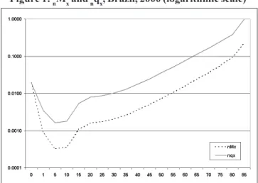
Figure 1 shows nqx and nMx. They are presented on a logarithmic scale because the magnitude of the range of these two indicators is such that it cannot be visualized on a single graph with an arithmetic scale. The two curves are parallel, except in the extreme ages where they coincide or start to join. In effect, the probability of dying consistently overesti-mates the mortality rate, except in the group of children less than 1 year of age, where nMx is above nqx. The two curves have the characteristic “J” shape, decreasing until the 5-9 interval, where they start to increase slightly until the 10-14 age group, then more rapidly until the 15 to 20 age group, and then regularly until they start joining at the 85-89 group.
Conclusion
Life tables present the mortality and survival experience of a whole population and permit evaluation of its effect on specific groups and over different periods. It is a simple in-strument that is easily constructed with data collected rou-tinely.
It is important to keep in mind that life tables are con-structed based on population data from censuses and mor-tality registries, and therefore that the quality limitations of the latter will also affect , to different degrees, the validity of the estimations from the life table.
Figure 1: nMx and nqx, Brazil, 2000 (logarithmic scale)
References:
(1) Pan American Health Organization. Area of Health Analysis and Information Systems. Techiques for the Measurement of the Impact of Mortality: Years of Potential Life Lost.
Epidemiological Bulletin. 24(2):1-4; 2003
(2) United States Bureau of the Census. Shryock H, Siegel JS et al.
(rev.). Washington, DC: United States Government Printing Office; 1973.
(3) Livi-Bacci M. Introducción a la demografía. Barcelona: Ed
Ariel; 1993.
(4) Chang CJ. Life Tables and Mortality Analysis. Geneva: World
Health Organization; 1980.
(5) Grundy EMD. Populations and population dynamics. In: Detels
R, Holland WW, McEwen JMc and Omenn GS Eds. Oxford
textbook of Public Health, vol 1. The Scope of Public Health. London: Oxford University Press; 1997.
(6) United States Census Bureau. Population Analysis Spreadsheets (PAS) [Internet page]. Available at: http://www.census.gov/ipc/ www/pas.html. Accessed on 5 December 2003.
Source: Prepared by Dr. Enrique Vázquez from PAHO’s Area of Health Situation Analysis and Information Systems (AIS) in the PAHO/WHO Argentina, Dr. Francisco Camaño (Universidad de Santiago de Compostela, Spain), Mr. John Silvi and Ms. Anne Roca (AIS - Washington, D. C.).
Ana V. Diez Roux
Divisions of Medicine and Epidemiology, Columbia University New York, New York, United States
PART II
A Glossary for Multilevel Analysis
EMPIRICAL BAYESESTIMATES
Estimates of parameters for a given group or higher lev-el unit (for example, estimates of group specific intercepts or slopes, such as b0j and b1j in equation (1), under MULTILEVEL MODELS) obtained by combining information from the group
itself with information from other similar groups investigat-ed.10, 19, 20 This is particularly useful when estimating parame-ters for a group with few within group observations. These estimates are “optimally” weighted averages that combine information derived from the group itself with the mean for all similar groups. The weighted average shifts the group specific estimate (derived using data only for that particular group) towards the mean for similar groups. The less precise the group specific estimate and the less the variability ob-served across groups, the greater the shift towards the over-all group mean. Thus, the estimate for a given group is based not only on its own data but also takes into account esti-mates for other groups and the characteristics groups share.20 Empirical Bayes estimates of parameters for a given group can be derived from multilevel models using estimates of the group level errors (for example, U0j and U1j , see MULTILEVEL MODELS) for that particular group. Empirical Bayes estimates
are also sometimes referred to as “shrinkage estimates” be-cause they “shrink” the group specific estimate towards the overall mean (although in fact when the overall mean is greater than the group specific estimate, the “shrunken” or empirical Bayes estimate may actually be greater than the group spe-cific estimate). In public health, empirical Bayes estimation can be used, for example, to derive improved estimates of rates of death or diseases for small areas with few observa-tions,21 or to estimate rates of different health outcomes for individual providers (hospitals, physicians, etc.)22 In other applications (which do not involve the structure of individu-als within groups although they are analogous to it),
empir-ical Bayes estimates of regression coefficients have been used to obtain improved estimates of associations in studies investigating the role of multiple exposures.23
ENVIRONMENTALVARIABLES
In the context of ecological studies and multilevel anal-ysis, the term “environmental variables” has sometimes been used to refer to group level measures of physical or chemical exposures. Environmental variables, so defined, have been proposed as a “type” of GROUPLEVELVARIABLE, distinct from DERIVEDVARIABLES and INTEGRALVARIABLES.11 These variables
are not derived by aggregating the characteristics of individ-uals but they do have group level and individual level ana-logues (for example, days of sunlight in the community and individual level sunlight exposure information). In contrast with derived and integral variables, which may be used as indicators of group level constructs, group level environ-mental variables are used exclusively as proxies for individu-al level exposures (which may be more difficult to measure for logistic or methodological reasons), rather than as indi-cators of a group level property, which is conceptually dif-ferent from the analogous measure at the individual level.
FIXEDEFFECTS/FIXEDCOEFFICIENTS
Regression coefficients (intercepts or covariate effects) that are not allowed to vary randomly across higher level units (see MULTILEVELMODELS). For example, in the case of
persons nested within neighborhoods, two options are avail-able for modelling the effects of neighborhood. One option is to include a dummy variable for each neighborhood. In this case the neighborhood coefficients are modelled as fixed (sometimes called “fixed effects”). Another option is to as-sume that the neighborhoods in the sample are a random sample of a larger population of neighborhoods and that the coefficients for the “neighborhood effect” vary randomly
(7) Xunta de Galicia, Consellería de Sanidade e Servicios Sociais. Organización Panamericana de la Salud. Area de Análisis de Situación y Sistemas de Información. Análisis Epidemiológico de Datos Tabulados (Epidat), version 3.0 [Computer Program for Windows]; [To be published]
(8) Coale, Ansley J, Demeny P. Regional Model Life Tables and
around an overall mean (for example, as reflected by Uoj in equation 2 under the entry for MULTILEVELMODELS). In this
case, the neighborhood effects are modelled as random (sometimes called “random effects”, see RANDOMEFFECTSMOD -ELS). In the same example, the coefficients for individual level
covariates can also be modelled as fixed or random. For ex-ample, if the relation between individual level income and blood pressure is not allowed to vary randomly across neigh-borhoods, the coefficient for individual level income is fixed (“fixed coefficient”). On the other hand, if the coefficient for individual level income is allowed to vary randomly across neighborhoods around an overall mean effect (as reflected by U1j in equation 3 under the entry for MULTILEVELMODELS),
the coefficient for income is modelled as random (sometimes called a “random coefficient”, see RANDOMCOEFFICIENTMOD -ELS). Although the terms “fixed effects” and “fixed
coeffi-cients “ are sometimes distinguished as noted above, they are often used interchangeably. Fixed effects models or fixed coefficient models are models in which all effects or coeffi-cients are fixed. See also RANDOMEFFECTS/RANDOMCOEFFI -CIENTS.
GROUPLEVELVARIABLES
Term used to refer to variables that characterize groups. The terms group level variables, macro variables and ecolog-ical variables are often used interchangeably.2, 6, 11, 14, 24 Group level variables may be used as proxies for unavailable or unreliable individual level data (for example, when neighbor-hood mean income is used as a proxy for the individual level income of individuals living in the neighborhood) or as indi-cators of group level constructs (for example, when mean neighborhood income is used as an indicator of neighbor-hood characteristics that may be related to individual level outcomes independently of individual level income). It is the second usage (as indicators of group level constructs) that is of particular interest in multilevel analysis. Group level variables have been classified into two basic types,11, 13, 24
DERIVEDVARIABLES and INTEGRALVARIABLES. Two additional
types of group level variables, STRUCTURALVARIABLES13 and ENVIRONMENTALVARIABLES11 are sometimes distinguished. The
term contextual variables has been used as a synonym for group level variables generally 6, 13 although it is sometimes reserved for derived group level variables.11, 14
HIERARCHICAL (LINEAR) MODELS
See MULTILEVELMODELS
INDIVIDUALLEVELVARIABLES
Term used to refer to variables that characterize individuals and refer to individual level constructs (for example, age or personal income).
INDIVIDUALISTICFALLACY
Term used as a synonym for the ATOMISTICFALLACY. May
sometimes also be used as a synonym for the PSYCHOLOGIS -TICFALLACY.
INTEGRALVARIABLES
A type of GROUPLEVELVARIABLE. Integral variables differ
from DERIVEDVARIABLES (another type of group level variable)
in that they are not summaries of the characteristics of indi-viduals in the group. Integral variables have no individual level analogues and necessarily refer to group level con-structs. Examples of integral variables include the existence of certain types of laws, political or economic system, social disorganization, or population density.11, 13 Integral variables have also been referred to as primary or global variables.
INTRACLASSCORRELATION
A measure of the degree of resemblance between lower level units belonging to the same higher level unit or clus-ter.25 In the case of individuals nested within groups (for example, neighborhoods), the intraclass correlation measures the extent to which values of the dependent variable are similar for individuals belonging to the same group. It can be thought of as the average correlation between values of two randomly drawn lower level units (for example, individuals) in the same, randomly drawn higher level unit (for example, neighborhood). It can also be defined as the proportion of the variance in the outcome that is between the groups or higher level units. In the case of a simple random intercept model, the intraclass correlation coefficient is estimated by the ratio of population variance between groups ( 00) to the total variance ( 00+ 2).25 (see
MULTILEVELMODELS) The
esti-mation of the intraclass correlation coefficient in models in-cluding random covariate effects, or in the case of non-nor-mally distributed dependent variables, is more complex and not always straightforward .
MARGINALMODELS
See POPULATION-AVERAGEMODELS.
MIXEDMODELS
Term used to refer to models that contain a mixture of FIXED EFFECTS (or fixed coefficients) and RANDOMEFFECTS (or
ran-dom coefficients). In mixed models some of the regression coefficients (intercepts or covariate effects) are allowed to vary randomly across higher level units but others are not (see MULTILEVELMODELS). Thus mixed models can be thought
other ways—that is, by modelling the correlations or covari-ances themselves rather than by allowing for random effects or random coefficients.26 These models (which are not multi-level models) have also been called covariance pattern mod-els,26 marginal models, or
POPULATIONAVERAGEMODELS.
MULTILEVELANALYSIS
An analytical approach that is appropriate for data with nested sources of variability—that is, involving units at a lower level or micro units (for example, individuals) nested within units at a higher level or macro units (for example, groups such as schools or neighborhoods).5, 10, 19, 24, 25, 27–30 Multilevel analysis allows the simultaneous examination of the effects of group level and individual level variables on individual level outcomes while accounting for the non-inde-pendence of observations within groups. Multilevel analy-sis also allows the examination of both between group and within group variability as well as how group level and indi-vidual level variables are related to variability at both levels. Thus, multilevel models can be used to draw inferences re-garding the causes of inter-individual variation (or the rela-tion of group and individual level variables to individual lev-el outcomes) but inferences can also be made regarding in-ter-group variation, whether it exists in the data, and to what extent it is accounted for by group and individual level char-acteristics. In multilevel analysis, groups or contexts are not treated as unrelated but are conceived as coming from a larg-er population of groups about which inflarg-erences want to be made. Multilevel analysis thus allows researchers to deal with the micro-level of individuals and the macro-level of groups or contexts simultaneously.5
Multilevel analysis has a broad range of applications in many situations involving nested sources of random vari-ability such as persons nested within neighborhoods,5, 30 patients nested within providers,31 meta analysis (observa-tions nested within sites),19, 32 longitudinal data analysis (re-peat measurements over time nested within persons),28, 33, 34 multivariate responses (multiple outcomes nested within in-dividuals),5 the analysis of repeat cross sectional surveys (multiple observations nested within time periods),35 the ex-amination of geographical variations in rates (rates for small-er areas nested within regions or largsmall-er areas)36 and the exam-ination of interviewer effects (respondents nested within in-terviewers).37 Multilevel analysis can also be used in situa-tions involving multiple nested contexts19, 28 (for example, multiple measures over time on individuals nested within neighborhoods) as well as overlapping or cross classified contexts (for example, children nested within neighborhoods and schools).38 The statistical models used in multilevel anal-ysis are referred to as MULTILEVELMODELS25, 28, 29 or
hierarchi-cal linear models.19, 39
MULTILEVELMODELS
The statistical models used in MULTILEVELANALYSIS.19, 25,
28, 29 The terms “hierarchical models” and “multilevel models” are often used synonymously. These models (or variants of them) have previously appeared in different literatures under a variety of names including RANDOMEFFECTSMODELS or RAN -DOMCOEFFICIENTMODELS40–42 “covariance components
mod-els” or “variance components modmod-els”,43, 44 and
MIXEDMOD -ELS.26 A simplified example for the case of a normally
distrib-uted dependent variable, a single individual level (lower lev-el unit) predictor and a single group levlev-el (higher levlev-el unit) predictor is provided below. Analogous models can be for-mulated for non-normally distributed dependent variables.10, 28, 39, 45
In the case of multilevel analysis involving two levels (for example, individuals nested within groups), the multilev-el modmultilev-el can be conceptualized as a two stage system of equations.
In the first stage (level 1), a separate individual level regression is defined for each group or higher level unit. (1) Yij = b0j + b1jIij + ij ij~ N(0, 2)
Yij= outcome variable for ith individual in jth group
Iij= individual level variable for ith individual in jth group b0j is the group specific intercept
b1j is the group specific effect of the individual level variable Individual level errors (eij) are assumed to be indepen-dent and iindepen-dentically distributed with a mean of 0 and a vari-ance of 2. The same regressors are generally used in all groups, but regression coefficients (b0j and b1j) allowed to vary from one group to another.
In a second stage (level 2), each of the group or context specific regression coefficients defined in equation (1) (b0j and b1j in this example) are modelled as a function of group level (or higher level) variables.
(2) b0j = 00 + 01Gj + U0j U0j ~ N(0, 00) (3) b1j = 10 + 11Gj + U1j U1j ~ N(0, 11)
cov(U0j, U1j) = 10
Gjgroup level variable
00 is the common intercept across groups
01 is the effect of the group level predictor on the group specific intercepts
10 is the common slope associated with the individual level variable across groups
11 is the effect of the group level predictor on the group specific slopes
dis-tributed with mean 0 and variances 00 and 11 respectively.
01 represents the covariance between intercepts and slopes. Thus, multilevel analysis summarizes the distribution of the group specific coefficients in terms of two parts: a “fixed” part that is common across groups ( 00 and 01 for the inter-cept, and 10 and 11 for the slope) and a “random” part (U0j for the intercept and U1j for the slope) that is allowed to vary from group to group (see also FIXEDCOEFFICIENTS and RANDOM COEFFICIENTS).
By including an error term in the group level equations (equations (2) and (3)), these models allow for sampling vari-ability in the group specific coefficients (b0j and b1j) and also for the fact that the group level equations are not determinis-tic (that is, the possibility that not all relevant macro-level variables have been included in the model). The underlying assumption is that group specific intercepts and slopes are random samples from a normally distributed population of group specific intercepts and slopes, or alternatively, that the macro errors are exchangeable—that is, that the residual variation in group specific coefficients across groups is un-systematic.10
An alternative way to present the model fitted in multi-level analysis is to substitute equations (2) and (3) in (1) to obtain:
Yij = 00 + 01Cj + 10Iij + 11CjIij + U0j + U1jIij + ij
The model includes the effects of group level variables ( 01), individual level variables ( 10) and their interaction ( 11) on the individual level outcome Yij. These coefficients ( 01, 10 and 11), which are common to all individuals regardless of the group to which they belong, are often called the FIXED COEFFICIENTS (or fixed effects). The model also includes a
ran-dom intercept component (U0j), and a random slope compo-nent (U1j). The values of these components vary randomly across groups, and hence U0j and U1j referred to as the RAN -DOMCOEFFICIENTS (or random effects). The parameters of the
above equations (fixed effects, random effects, variances of the random effects, and residual variance) are simultaneous-ly estimated using iterative methods. The level 1 and level 2 variances ( 2,
00, 11 , 10) are called the (CO)VARIANCECOMPO
-NENTS.
Many variants of the more general model illustrated above are possible. For example, only group specific inter-cepts (b0j) may be modelled as random (these models have also been called RANDOMEFFECTSMODELS). When covariate
effects (b1jin the example above) are modelled as random these models have also been called RANDOMCOEFFICIENTMOD -ELS. When some of the coefficients are fixed and others are
random, these models have also been called “mixed effects models” or simply MIXEDMODELS. When all coefficients are
modelled as fixed (no random errors are included in level 2 equations), these models are reduced to traditional CONTEX
-References:
NOTE: References 1-18 were included in Part I of the Glossary, in Vol. 24,
No. 3 (2003) of the Epidemiological Bulletin.
(19) Bryk AS, Raudenbush SW. Hierarchichal linear models: applications and data analysis methods.Newbury Park: Sage, 1992.
(20) Rice N, Jones A. Multilevel models and health economics. Health Econ 1997;6:561–75.
(21) Clayton D, Kaldor J. Empirical Bayes estimates of age-standardized relative risks for use in disease mapping. Biometrics 1987;43:671–81. (22) Thomas N, Lonford N, Rolph J. Empirical Bayes methods for estimating
hosptial-specific morality rates. Stat Med1994;13:889–903.
(23) Witte JS, Greenland S, Haile RW, et al. Hierarchical regression analysis applied to a study of multiple dietary exposures and breast cancer.
Epidemiology 1994;5:612–21.
(24) Von Korff M, Koepsell T, Curry S, et al. Multi-level research in epidemiologic research on health behaviors and outcomes. Am J Epidemiol 1992;135:1077–82.
(25) Snijders TAB, Bosker RJ. Multilevel analysis: an introduction to basic and advanced multilevel modeling. London: Sage, 1999.
(26) Brown H, Prescott R . Applied mixed models in medicine. New York: Wiley, 2000.
(27) Mason W, Wong G, Entwisle B. Contextual analysis through the multilevel linear model. In: Leinhardt S, ed. Sociological methodology. San Francisco: Josey Bass, 1983–1984: 72–103.
(28) Goldstein H. Multilevel statistical models. New York: Halsted Press, 1995.
(29) Kreft I, deLeeuw J. Introducing multilevel modeling. London: Sage, 1998.
(30) Diez-Roux AV. Multilevel analysis in public health research. Annu Rev Public Health 2000;21:171–92.
(31) Sixma HJ, Spreeuwenberg PM, Pasch MAvd. Patient satisfaction with the general practitioner: a two-level analysis. Med Care 1998;36:212–29. (32) Hedeker D, Gibbons R, Davis J. Random regression models for
multicenter clinical trials data. Psychopharmacol Bull1991;27:73–7. (33) Rutter C, Elashoff R. Analysis of longitudinal data: random coefficient
regression modelling. Stat Med1994;13:1211–31.
(34) Cnaan A, Laird NM, Slasor P. Using the general linear mixed model to analyse unbalanced repeated measures and longitudinal data. Stat Med
1997;16:2349–80.
(35) DiPrete T, Grusky D. The multi-level analysis of trends with repeated cross-sectional data. Sociol Methodol 1990;20:337–68.
(36) Langford I, Bentham G, McDonald A. Multi-level modelling of geographically aggregated health data: a case study of malignant melanoma mortality and uv exposure in the European community. Stat Med1998;17:41–57.
(37) Hox JP, de Leeuw ED, Kreft IGG. The effect of interviewer and respondent characteristics on the quality of survey data: a multilevel model. In: Biemer PP, Lyberg LE, Mathiowetz NA, et al, eds.
Measurement errors in surveys. New York: Wiley, 1991.
(38) Goldstein H. Multilevel cross-classified models. Sociol Methods Res
1994;22:364–75.
Source: Published initially as “A glossary for multilevel analysis” in the Journal of Epidemiology and Community Health, 56:588-594, 2002.
TUALEFFECTSMODELS. Multilevel models can also account for
Revision of the International Health Regulations
Background
The International Health Regulations (IHR) represents the earliest multilateral initiative by countries to develop an effective framework to prevent cross-border transmission of diseases. The IHR strives to harmonize public health, trade, and traffic, and today remains the only binding set of regula-tions on global surveillance for infectious diseases by the World Health Organization’s (WHO) Member States.
The current IHR was adopted in 1969, amended in 1973 with additional provisions for cholera, and subsequently re-vised in 1981 to exclude smallpox. Today, only cholera, plague and yellow fever are notifiable diseases under the IHR. Its fundamental purpose is to ensure maximum security against the international spread of diseases with a minimum inter-ference with world traffic.
Because of extensive globalization in travel and trade, diseases from even remote parts of the world could spread to other areas. Potentially damaging traffic and trade embar-goes may be imposed, sometimes based only on the percep-tion of risk for disease importapercep-tion, and potentially reach glo-bal proportions as happened during the cholera epidemic in the Americas in the early 1990’s.
To address the threat posed by substantial increases in international travel and the potential for the rapid spread of infectious diseases, especially by air travel, the World Health Assembly (WHA) requested the revision of the Internation-al HeInternation-alth Regulations (IHR) in the 1995 resolution WHA 48.7.
Progress
The current revision is a collaborative process that was initiated in 1995. Its essence is to review the gaps in the present IHR and transform it into an effective regulatory tool for WHO Member States to strengthen global disease sur-veillance and to be proactive in dealing with international outbreaks. Proposed changes are being developed and fine-tuned to adapt to contemporary global surveillance demands and control of international outbreaks. All of the items intro-duced are proposals, and as such require extensive consulta-tion before presentaconsulta-tion to the WHA and ultimate accep-tance by Member States.
The revision approach is based on three specific principles1: – Ensuring that all public health risks (mainly of infectious origin) that are of urgent international importance are reported under the Regulations
– Avoiding stigmatization and unnecessary negative im-pact on international travel and trade and invalid report-ing from sources other than Member States, which can have serious economic consequences for countries
– Ensuring that the system is sensitive enough to detect new or re-emerging public health events.
To this end, three key changes are being proposed. First, the scope of reported events will be expanded to include all
public health emergencies of international concern. There will be a clear link between reporting and established mecha-nisms for action.
To define an event as a public health emergency of inter-national concern a set of specific criteria is being proposed: (1)Severity: The health event produces an abnormal increase
of case fatality and/or incidence rates
(2)Unusual or unexpected: An emerging health event or a known health event showing an abnormal behavior (3) Risk of international propagation
(4) The event will lead, eventually, to international restric-tions of travel and trade
Second, a National Focal Point will be designated to facilitate the greater flow of information between the WHO and the different national levels in both directions. Specifi-cally, this focal point should be able to: manage international surveillance and response requirements; advise senior health officials regarding notification to the WHO, and implementa-tion of WHO recommended measures, distribuimplementa-tion of infor-mation, and coordination of input from several key national areas, such as disease surveillance, ports, airports, and ground crossings’ public health services, as well as other government departments, such as agriculture and customs; and finally, act as the technical resource coordinating body during the revision and implementation processes.
Third, core country capacities required in surveillance and response, including at points of entry will be defined and included in the IHR. In order for urgent national events to be picked up early, each country will require a surveillance system informing on unusual and unexpected events from the periphery into the center in a very short time, including the capacity to analyze rapidly such data. In many countries, this surveillance/analysis capacity may already be in place. Others may need a grace period to fulfill this future IHR re-quirement, and external assistance and funding may become necessary.
The 43rd Meeting of the Pan American Health Organiza-tion (PAHO) Directing Council adopted ResoluOrganiza-tion CD43.R13 in support of the revision of the International Health Regula-tions (IHR), urging Member States to participate actively in the review process both nationally and through the regional integration systems.