Bol. Ciênc. Geod. vol.20 número2

BCG - Boletim de Ciências Geodésicas - On-Line version, ISSN 1982-2170

http://dx.doi.org/10.1590/S1982-21702014000200018

A STUDY OF THE CHILEAN VERTICAL NETWORK

THROUGH GLOBAL GEOPOTENTIAL MODELS AND THE

CNES CLS 2011 GLOBAL MEAN SEA SURFACE

Um estudo da rede vertical chilena através do modelo geopotencial global e do CNES CLS 2011 superfície global média do oceano

HENRY MONTECINO CASTRO1 AHARON CUEVAS CORDERO1 SÍLVIO ROGÉRIO CORREIA DE FREITAS2

1_{Department of Geodetic Science and Geomatics}

University of Concepcion, Los Angeles, Chile 2

Geodetic Reference Systems and Satellite Altimetry Laboratory Geodetic Sciences Graduation Course - Federal University of Paraná, Brazil

henrymontecino@gmail.com; aharon.cc@gmail.com; sfreitas@ufpr.br

ABSTRACT

relation to different GGMs. The results showed consistency between the values obtained by the two methods at the TG of Valparaíso and Puerto Chacabuco. In terms of the evaluation of the GGM, GOEGM08 produced the best results.

Keywords: Vertical Network; Global Geopotential Models; Mean Dynamic

Topography.

RESUMO

A maioria dos aspectos relacionados com a componente horizontal do Sistema de Referencia para as Americas (SIRGAS) tem sido resolvidos. No entanto, no caso da componente vertical, ainda existem aspectos de definição, realizações nacionais e unificação dos sistemas de altitudes continentais ainda não resolvidos. O Chile não é exceção; devido às suas características geográficas especiais uma série de marégrafos (TG) tiveram que ser instalados a partir das linhas de nivelamento que compõem a Rede Vertical chilena (CHVN). Este estudo explorou os afastamentos do CHVN por duas abordagens diferentes, uma geodésica e outra oceanográfica. Na primeira abordagem, os afastamentos foram obtidos em relação aos seguintes Modelos do Geopotencial Global (MGGs): o modelo somente satélite (com consistência global) GO_CONS_gcf_2_tim_r3 derivado da missão GOCE; o EGM2008 (combinado com dados oriundos de diferentes SGRs) e GOEGM08, combinando informações do GO_CONS_gcf_2_tim_r3 em longos comprimentos de onda (nmax~200), com médios e curtos comprimentos de onda do EGM2008 (n>200). No método oceanográfico foi utilizado o MSS CNES CLS 2011 Global Mean Sea e o EIGEN_GRACE_5C para obter os valores de MDT nos diferentes TG. Também foi avaliada a CHVN em relação a diferentes MGG. Os resultados mostraram consistência entre os valores obtidos pelos dois métodos no TG de Valparaíso e Puerto Chacabuco. Em termos de avaliação do GGM, o GOEGM08 produziu os melhores resultados.

Palavras-chave: Rede Vertical; Modelos do Geopotencial Global; Topografia do

Nível Médio do Mar.

1. INTRODUCTION

In the current paradigms of the International Earth Rotation and Reference System Service (IERS), its Terrestrial Reference Frames (ITRFs) are realized based on various techniques from Space Geodesy like: GNSS (Global Navigation Satellite

System); VLBI (Very Long Baseline Interferometry); SLR (Satellite Laser Ranging);

LLR (Lunar Laser Ranging); and DORIS (Doppler Orbitography and

Radiopositioning Integrated by Satellite). In the last two decades several continental

fileadmin/images/SIRGAS-CON-D.pdf). Nowadays, it is possible to establish only one Geodetic Reference System (GRS), since the global to local horizontal networks are consistent. However, the heights in these networks are realized without physical meaning. Related to this context, the main scientific research subject of SIRGAS project is related to the establishment of one unified height system in Latin America with physical meaning (SÁNCHEZ, 2009). Similar task is also in the context of the Inter Commission Project 1.2 (ICP 1.2) of the International Association of Geodesy (IAG) because there are more than 100 height systems in the world without consistency with a World Height System – WHS (SIDERIS et al., 2011).

Aspects of definition and realization of a WHS, and its connection with local height systems are current global challenges. Latin America is no exception. In order to solve these problems the SIRGAS project defined its main purpose of its Working Group III (WGIII) (see http://www.sirgas.org/index.php?id=56): to define one consistent height system in Latin America. They will choose one consistent height system with physical meaning and in connection with the SIRGAS-CON GNSS stations; to promote the modernization of national vertical networks by adoption of geopotential numbers along with each national vertical network. This approach is fundamental for connecting continental vertical networks based in geopotential numbers and for establishing the relationship of each national vertical datum with one WHS for one reference epoch.

As in most countries in South America, Chile has an ambiguous height system. Aspects such as the epoch of definition, type of height and tidal system are not clearly described (SÁNCHEZ, 2011).

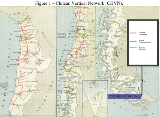
Due to some geographic Chilean characteristics such as extension and shape, different networks linked to the tide gauges (TG) of Arica, Antofagasta, Valparaíso, San Antonio, Talcahuano, Puerto Montt and Punta Arenas (Maturana & Barriga, 2001) was realized the Chilean Vertical Network (CHVN) mainly. The CHVN was measured at different epochs and many TG are not yet linked. Also, most of the leveling lines that compose the CHVN were leveled before 1980, and some of these lines were leveled again to determine possible variations caused by the 1960, 1965 and 1985 earthquakes (MATURANA & BARRIGA, 2001). Fig. 1 shows the configuration and the periods in which the lines were measured.

It must be noted that only the most recent leveling lines (in green) are freely available, and are the only ones used in this study.

The CHVN was established from different TGs and in different epochs; so it can be interpreted as height systems with different realization, and with inconsistencies among its different segments. The predominant component in this inconsistency is generally attributed to the Mean Dynamic Topography (MDT), also denoted as Sea Surface Topography (SSTop) (FILMER & FEATHERSTONE, 2012). The MDT is the discrepancy between the Mean Sea Level (MSL) and the geoid observed between two epochs (HECK & RUMEL, 1989), and may reach values up to ±2.0 m (ENGELIs, 1985; ENGELIS, 1987; RIO & HERNÁNDEZ, 2004). This large difference is generated by geostrophic dynamic equilibrium of the ocean currents, which result from factors such as wind, changes in salinity, local resonances, temperature and pressure that are directly related to the Earth System dynamic aspects. The MDT may be defined by the Mean Sea Surface (MSS) height and from the geoid height (N) as (BOSCH, 2002):

N MSS

MDT = − (1)

A number of MDT models have been developed, including: MSS93A (ANZENHOFER & GRUBER, 1995), WHU2000 MSS (WEIPING et al., 2003), CLS_SHOM98 (SCHAEFFER et al., 1998), the model of Cazenave et al., 1996, KMS04 (ANDERSEN et al., 2005), GSFC00 (WANG, 2001), CLS01 (HERNANDEZ & SCHAEFFER, 2001), DNSC08 (ANDERSEN & KNUDSEN, 2009) and CNES CLS 2011 (SCHAEFFER et al., 2012). The CNES CLS 2011 Global Mean Sea surface was used in this study since it is one of the newest models, based on 16 years of observation (1993-2009) by different altimeter satellites missions, and provides a resolution of 2’ (SCHAEFFER et al., 2012).

FLURY, 2006). It is very important to mention the EGM2008 (PAVLIS et al., 2012) reaches the harmonic degree and order (n/m) of 2190 and 2159 respectively. The discrepancies between geoid heights computed from EGM2008 and those computed from independent GPS/Leveling data are on the order of 5 cm to 10 cm where high quality gravity data is available (PAVLIS et al, 2012). However, in region with poor gravity data distribution, the EGM2008 referred discrepancies can reach up 50 cm, since it combines satellite and terrestrial information, the latter reduced to different equipotential surfaces because of unknown local datums effects (e.g. on gravity anomalies) or gravity anomalies filled mainly by RTM technique as is the case of Chile and most of South America.

It must be noted that the main mission objectives of GOCE is to contribute to the global unification of height systems by producing “unbiased” gravity field models (ESA, 1999). The current expectation of the GGMs of GOCE in a resolution of 85 km is an error on the order of 3 cm (GATTI et al., 2012), and for shorter wavelengths, omission errors of up to 30 cm (GERLACH & RUMMEL, 2012). Combinations of satellite-only GGM with Digital Elevation Models (DEM) information may provide less biased models, and as a result more adequate to be used in the unification of height systems (e.g. MONTECINO et al., 2011, GATTI et al., 2012). A number of methodologies have been used to evaluate the performance of the GGM; the most commonly used is the comparison between the geoid height (NMGG) obtained from the GGM and the geoid height (NGPS/BM) obtained by GPS ellipsoidal height determination on spirit leveling benchmarks (BMs) (c.f. MERRY, 2007; AMOS & FEATHERSTONE, 2003; FEATHERSTONE, 2001; RODRÍGUEZ et al., 2006; SIDERIS et al., 1992). This comparison should provide a systemic offset component for every realization of a height system, remembering that part of the offset is associated with the quality of the GGM.

So far there have been no studies of the deformation/inconsistency of the CHVN due to the spatio-temporal effect of the MDT. It must be noted that in addition to the MDT, there are a serie of factors that could contribute to the inconsistency of the CHVH, such as systematic errors in leveling, discrepancies between different gravimetric reductions and vertical movements. However, in this study only the contribution of the MDT is considered.

The following will be an exploration of the different offset levels of the CHVN by using oceanographic and geodetic methodologies. We will also explore the offsets of the GGMs GOCE and EGM2008 in relation to the CHVN.

2. DATA AND METHODS

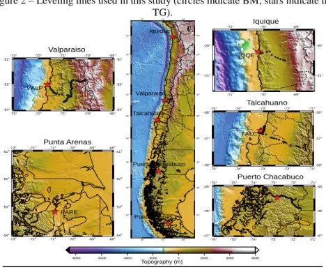
This study was performed along the entire extension of Chile, specifically in the 5 zones indicated in Fig. 2.

following data of the leveling lines were obtained from the publication “Red

Nacional de Gravedad RNG-CHILE, 2009”:

• Line 4A: Iquique-Humberstone

• Line 5A: Matilla-Pica

• Line 6A: Huara-Est. Lagunas

• Line 11ª: Ruta 5-Matilla

• Line 19E: San Bdo.-Valparaíso

• Line 12E: Los Andes-Esc. De Montaña

• Line 9E: Colina-Los Andes

• Line 24E: San Antonio-Santiago

• Line 10G: Dichato-Tigo

• Line 8G: Talcahuano-Antuco

• Line 6I, 7I: Chacabuco-Huemules

• Line 6L, 5L: Punta Arenas-Cabeza de Mar-Monte Aymond In addition, the following models were used:

EGM2008 (PAVLIS et al., 2008), was obtained from the International Center Global Earth Model (ICGEM).

The go_cons_gcf_2_tim_r3 (PAIL et al., 2011), was obtained from the International Center for Global Earth Model (ICGEM), with n/mmax=250.

The Mean Dynamic Topography model DNSC08 MDT (ANDERSEN & KNUDSEN, 2009) was obtained from the site http://www.space.dtu.dk/english/ Research/Scientific_data_and_models/downloaddata.

The Global Mean Sea Surface MSS CNES CLS2011 (SCHAEFFER et al., 2012) was obtained from website htp://www.aviso.oceanobs.com/en/data/products/ auxiliary-products/mss.html.

A evaluation of the performance of MDT’s models: DNSC08, CNES CLS 2011, DTU10 and DTU12 in relation of tide gauge observations was carried out. In this experiment, the CNES CLS 2011 and DTU12 models give the best results; however, the DTU12 model does not provide data for the Puerto Chacabuco tide gauge. Therefore, the MSS CNES CLS 2011 was used in this study (see table 1).

Table 1 – Behavior of the MDT models R.M.S. (m) TG-CNES CLS 2011 1.474

TG-DTU10 1.980

TG-DNSC08 1.872

Figure 2 – Leveling lines used in this study (circles indicate BM; stars indicate the TG). -76° -76° -72° -72° -68° -68° -52° -52° -48° -48° -44° -44° -40° -40° -36° -36° -32° -32° -28° -28° -24° -24° -20° -20° Valparaiso Talcahuano Puerto Chacabuco Iquique Punta Arenas -73° -73° -72° -72° -71° -71° -70° -70° -69° -69° -68° -68° -54°

-53° -53°

-52° -52°

-51° -76° -76° -75° -75° -74° -74° -73° -73° -72° -72° -71° -71° -47° -46° -46° -45° PARE -45° -47° -51° -54° PCHA

-8000 -6000 -4000 -2000 0 2000 4000 6000

Topography (m) Punta Arenas Puerto Chacabuco -73° -73° -72° -72° -71° -71° -70° -70° -69° -69° -34° -33° -33° -32° -32° -34° Valparaiso -75° -75° -74° -74° -73° -73° -72° -72° -71° -71° -38° -37° -37° -36° VALP -36° -38° Talcahuano -71° -71° -70° -70° -69° -69° -21° -21° -20° -20° TALC Iquique IQQE

2.1 Determination of the offset of the CHVN by using a GGM

The determination of the mean offset between the local reference level of every realization of the CHVN and a GGM (e.g. EGM2008) was based on the approach by Bursa et al., (2001) by using the following equation:

(

)

∑

i h N H

n ₁

1

(2)

where I is the offset between datum I and the GGM; hk is the ellipsoidal height at point k; Nk is the geoid height referred to the GGM in the point k; Hki is the height linked to the LMSL in the point k; n is the number of points.

The equation used to estimate the reference geoid height at the local reference level was:

H h

NGPS/BM = − (3)

The difficulties in determining the offset using GGM are associated mainly with the spatial resolution of these models, especially the satellite-only GGM, which are free of local reference frames (unbiased). Combined models such as the EGM2008 have a high resolution (nmax~2190); however, these models can be biased because the dependency on data coming from different reference frames. The EGM2008 is indirectly linked to different equipotential surfaces and several strategies are applied aiming to reduce local effects (PAVLIS et al., 2012), since it involves terrestrial observations reduced to different datum. There are other approaches to improve the resolution of the satellite-only GGMs, which are not strongly affected by local reference frames, for example, recovery of the short wavelength part from classical computation of the residual geoid signal by the Stokes integral formula using terrestrial mean gravity anomalies, i.e. by the solution of the Geodetic Boundary Value Problem, or from a high resolution global gravity model, such as EGM2008 (RUMMEL, 2012). A similar approach was applied by Gatti et al., (2012). In this research we use an expanded GOCE satellite-only GGM up to nmax~200, and the short wavelength part obtained from the EGM2008, is

∑ ∑

∑ ∑

L P T P T S P T S P

T P

T (4)

where, n and m are degree and order, T(P) is the disturbing potential of a point P,

TL(P) is the component of the disturbing potential recovered by a satellite-only

GGM (normally expanded nmax~200), and TH(P) is the residual component obtained from a combined high-resolution GGM. It is important to note that the component

TH(P) has a negligible bias.

Two scenarios were tested in this study. In the first, only the EGM2008 in its maximum expansion was used. The second method used is based on the approach of equation 4, based on this, the GOEGM08 model was constructed using low coefficients (n≤200) of go_cons_gcf_2_tim_r3 unbiased GOCE model and high coefficients (201≤n≤2190) of EGM2008.

2.2 Determination of the offset of the CHVN by an oceanographic approach

To evaluate the consistency of the MDT in the neighborhood of the TG with the offsets obtained from equation 2, we used the following comparison:

i

i−SSTop

∆ =

δ (5)

the TG were obtained by Krigging method in the form Point kriging with linear variogram model without a drift.

3. RESULTS AND DISCUSSION

The offsets obtained from equation 2 showed a variable behavior in values as well as in tendencies as a function of the reference equipotential surface from a GGM; these are shown in Fig. 3. However, considering that the MSS CNES CLS 2011 is referred to EIGEN_GRACE_5C GGM, a change of reference surface was applied in order to refer it to the EGM2008, the same reference surface for every offset calculated. Using the latter comparison for the five regions, the IQQE, VALP and PCHA regions showed the same tendency, noted that in PCHA, the offset and the MDT are highly consistent (see Tab. 2). However, TALC and PARE showed large differences with opposite tendencies. The CNES CLS 2011 and DNSC08 models present the same tendencies; however, these provide values significantly different between them.

Table 2 – Comparison of offset by oceanographic approach. EGM2008 vs

DNSC08 (cm)

EGM2008 vs CNES CLS 2011 (cm)

IQQE 42 16

VALP -2 -51

TALC -45 -99

PCHA 6 0

PARE 138 49

Figure 3 – Offset for each region (tide gauge) by oceanographic and GGM (EGM2008) approaches.

1 2 3 4 5

-150 -125 -100 -75 -50 -25 0 25 50 75 100 125 150

Tide Gauge

S

S

T

o

p

(

c

m

)

SSTop(GPS/BM-EGM2008) SSTop(DNSC08) SSTop(CNES CLS11) SSTop(GPS/BM-GOCE) SSTop(GPS/BM-GOEGM08)

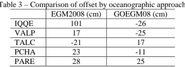
Based on Fig. 3, the GGMs which best adapt to the CHVN are EGM2008 and GOEGM08. The EGM2008 showed better adaptation in the central and southern regions of Chile, including the zones of VALP, TALC, PCHA y PARE. However, in northern region (IQQE) has a difference that is significantly higher. The GOEGM08 showed better performance than EGM2008 for all regions evaluated (see Tab. 3).

Table 3 – Comparison of offset by oceanographic approach. EGM2008 (cm) GOEGM08 (cm)

IQQE 101 -26

VALP 17 -25

TALC -21 17

PCHA 23 -11

PARE 28 25

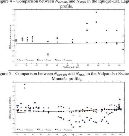
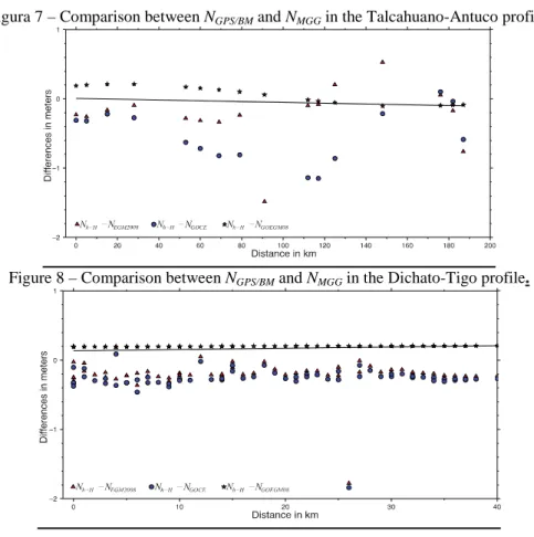
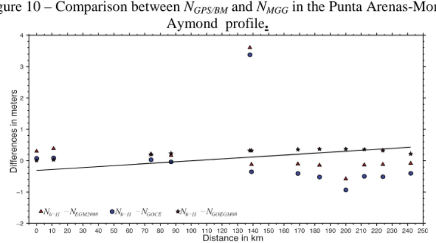
In addition to the evaluation by zones (e.g. Iquique, Valparaíso), we also evaluated by profiles in north-south (N-S) and east-west (E-W) directions, to explore the inclinations of the GGMs related to the CHVN. Due to the large dispersion of the data with respect to the lines fitted in the EGM2008 and go_cons_gcf_2_tim_r3 models, these were not considered. However, the data of the GOEGM08 model showed a very good consistency with the adjusted lines (see Fig. 4 to Fig. 9). The inclinations estimated for the profiles of Iquique- Est. Laguna (E-W), Valparaíso-Esc. Montaña (E-(E-W), San Antonio-Los Andes (N-S), Talcahuano-Antuco (E-W), Dichato-TIGO (N-S), Chacabuco-Huemules (E-W) and Punta Arena-Cabeza de Mar (N-S) were -4 mm/km, 2.0 mm/km, 1.0 mm/km, -2.0 mm/km, 0.5 mm/km, -0.3 mm/km and 1.0 mm/km, respectively. Considerable inclinations in both the N-S and E-W profiles were observed to not have a clear tendency in any particular direction.

Figure 4 – Comparison between NGPS/BM and NMGG in the Iquique-Est. Lagunas profile.

Figure 5 – Comparison between NGPS/BM and NMGG in the Valparaíso-Escuela de Montaña profile.

Figura 7 – Comparison between NGPS/BM and NMGG in the Talcahuano-Antuco profile.

Figure 8 – Comparison between NGPS/BM and NMGG in the Dichato-Tigo profile.

Figure 10 – Comparison between NGPS/BM and NMGG in the Punta Arenas-Monte Aymond profile.

4. SUMMARY

An exploratory investigation about inconsistencies of the Chilean height system is presented. The determination of the offset of the CHVN in relation to a reference surface was explored using a geodetic and an oceanographic approach. The values obtained showed high consistency between the DNSC08 model and the offsets (linked to EGM2008) only in VALP and PCHA TGs, whereas the offsets obtained from the CNES CLS 2011 are consistent in IQQE and PCHA TGs. Also, a tailored model was constructed using the long wavelengths of the go_cons_gcf_2_tim_r3 and short wavelengths from EGM2008 component called GOEGM08. However, the hybrid GOEGM08 model obtained of the low coefficients (n<200) of GOCE and the high coefficients of EGM2008 showed a great improvement over that of these models separately, as well as remaining an unbiased model. Moreover, it was noted that the GOEGM08 shows the best adaptation to the segments of the CHVN and, this model presents the best fit relative to the NBM/EGM2008. It must be emphasized that the study was strongly limited by lack of data (consistent gravimetric information, regional geoid, etc.); thus our approach used mainly global models and freely available data (BMs, geodetic coordinates).

Some aspects of vertical reference frame (definition of the reference point and others) and line setting (constraining links in the network adjustment, number of reference tide gauges, types of height, gravimetric reductions, MDT reduction, reductions for crust movements and others) of the Chilean Height System were not covered, because of either lack of information, diffuse information or a negligible effect in our context.

In spite to the limitations mentioned, this study gives an idea of the current situation of the Chilean Height System.

REFERENCES

ALTAMIMI, Z., BOUCHER, C., AND SILLARD, P. (2002a). “New Trends for the Realization of the International Terrestrial Reference System,” Adv. Space

Res., 30, No. 2, pp. 175–184.

ANGERMANN, D., DREWES, H., GERSTL, M., KRÜGEL, M., AND MEISEL, B. (2009). Geodetic Reference Frames, in: H. Drewes (eds). DGFI Combination Methodology for ITRF2005 Computation, p 11–16, IAG symposia 134, Springer.

ALTAMIMI, Z., P. SILLARD, AND C. BOUCHER (2002b), ITRF2000: A new release of the International Terrestrial Reference Frame for earth science applications, J. Geophys. Res., 107(B10), 2214, doi:10.1029/2001JB000561. AMOS, M. J. AND FEATHERSTONE, W. E. (2003). Comparisons of Recent

Global Geopotential Models with Terrestrial Gravity Field Observations Over New Zealand and Australia. Geomatics Research Australasia 79: 1-20. ANDERSEN, O. B., VEST, A. L. AND KNUDSEN, P. The KMS04 Multi-Mission

Mean Sea Surface. Proceedings of the Workshop: GOCINA: Improving Modelling of Ocean Transport and Climate Prediction in the North Atlantic Region Using GOCE Gravimetry: April 13 - 15, 2005, Novotel, Luxembourg-Kirchberg; Grand-Duchy of Luxembourg.

ANDERSEN, O. B., AND P. KNUDSEN (2009), DNSC08 mean sea surface and mean dynamic topography models, J. Geophys. Res., 114, C11001, doi:10.1029/2008JC005179.

ANZENHOFER, M., AND GRUBER, T. (1995). MSS93A: A new stationary sea surface combining one year upgraded ERS 1 fast delivery data and 1987Geosat altimeter data. Bull. Geod., 69, 157-163.

BOSCH, W. The Sea Surface Topography and its Impact to Global Height System Definition. International Association of Geodesy Series, v. 124 (Vertical Reference Systems), p. 225-230, Berlin: Springer, 2002.

BURŠA M., KOUBA J., MÜLLER A., RADĚJ K., TRUE S.A., VATRT V. AND VOJTÍŠKOVÁ M. (2001). Determination of geopotential differences between local vertical datums and realization of a World Height System. Stud.

Geophys. Geod., 45, 2001, 127−132.

CAZENAVE, A., SCHAEFFER, P., BERGE, M., BROSSIER, C., DOMINH, K. AND GENNERO, M.C. (1996). High-resolution mean sea surface computed withvaltimeter data of ERS-1 (geodetic mission) and TOPEX-POSEIDON,

Geophys. J. Int., 125, 696-704.

EKMAN, M. (1989). Impacts of geodynamic phenomena on systems for height and gravity. Bulletin Geodesique 63:281-296.

ENGELIS, T. (1985). Global circulation from Seasat altimeter data. Marine

ENGELIS, T. (1987). Spherical harmonics expansion of the Levitus Sea Surface

Topography. Report No. 385, Department of Geodetic Science and Surveying,

The Ohio State University, Columbus, Ohio.

ESA (1999) Gravity field and steady-state ocean circulation mission. Report for

mission selection of the four candidate earth explorer core missions. SP

1233(1) ESA

FILMER, M. S. AND FEATHERSTONE, W. E. (2012) A Re-Evaluation of the Offset in the Australian Height Datum Between Mainland Australia and Tasmania. Marine Geodesy, 35:1, 107-119.

FEATHERSTONE, W. E., 2001. Absolute and relative testing of gravimetric geoid models using Global Positioning System and orthometric height data.

Computers and Geosciences, 27: 807-814.

FLURY, J. (2006). Short-wavelength spectral properties of the gravity field from a range of regional data set. Journal of Geodesy, 79: 624-640.

GATTI, A., REGUZZONI, M. AND VENUTI, G. (2012). The height datum problem and the role of satellite gravity models. Journal of Geodesy,1-8. doi: 10.1007/s00190-012-0574-3.

GERLACH, C. AND RUMMEL, R. (2012). Global height system unification with GOCE: a simulation study on the indirect bias term in the GBVP approach.

Journal of Geodesy, 1-11.

HECK, B. & RUMMEL, R. (1989). Strategies for solving the vertical Datum

problem using terrestrial and satellite geodetic data. Sea Surface Topography

and the Geoid. International Union of Geodesy and Geophysics. International Association of Geodesy.

HERNANDEZ, F. AND SCHAEFFER, P. (2001). The cls01 mean sea surface: A validation with the gsfc00.1 surface, Tech. rep., CLS Ramonville St Agne., 14 pp.

MATURANA R. AND BARRIGA, R. The Vertical Geodetic Network in Chile. In: Drewes, H., Dodson, A., Fortes, L.P.S., Sánchez, L. and Sandoval, P. (Ed.):

Vertical Reference Systems, Springer, IAG Symposia; Vol. 124: 23-26, 2001.

MERRY, C. (2007). Evaluation of global geopotential models in determining the quasi-geoid for Souther. Survey Review, Volume 39, Number 305, pp. 180-192(13)

MONTECINO, H., DE FREITAS, S. R. AND JAMUR, K. Connection of Imbituba and Santana Brazilian Vertical Datums based on Satellite Gravimetry and Residual Terrain Model. International Union of Geodesy and Geophysics

(IUGG) General Assembly, 2011, Melbourne, Australia.

MONTECINO, H., CUEVAS, A., ROBLES, O. AND DE FREITAS, S. R. (2013). Evaluation of some Mean Dynamic Topography models for unifying the frames in the Chilean Height System. VIII Colóquio Brasileiro de Ciências

Geodésicas. December 2-5, Curitiba, Brazil.

ABRIKOSOV, O., VEICHERTS, M., FECHER, T., MAYRHOFER, R., KRASBUTTER, I., SANSÒ,F. AND TSCHERNING, C. (2011). First GOCE gravity field models derived by three different approaches. Journal of

Geodesy, 85: 819-843.

PAVLIS, N. K., S. A. HOLMES, S. C. KENYON, AND J. K. FACTOR (2012). The development and evaluation of the Earth Gravitational Model 2008 (EGM2008), J. Geophys. Res., 117, B04406, doi:10.1029/2011JB008916. RIO, M.-H., AND F. HERNANDEZ (2004), A mean dynamic topography

computed over the world ocean from altimetry, in situ measurements, and a geoid model, J. Geophys. Res., 109, C12032, doi:10.1029/2003JC002226. RODRIGUEZ-CAZEROT, G., LACY, M.C., GIL, A.J. AND BLAZQUEZ, B.

(2006). Comparing recent geopotential models in Andalusia (southern Spain).

Studia Geophysica et Geodaetica, 50: 619-631.

RUMMEL, R. (2012). Height unification using GOCE. Journal of Geodetic

Science. Volume 2, Issue 4, Pages 355–362.

SCHAEFFER, P., HERNANDEZ, F., LE TRAON, P.-Y., MERTZ, F. AND BAHUREL, P. ( 1998). A Mean Sea Surface dedicated to Ocean Studies:

Global Estimation. Poster Session EGS Nice, France, Apr.

SCHAEFFER P., Y. FAUGERE, J. F. LEGEAIS, A. OLLIVIER, T. GUINLE, N. PICOT (2012), The CNES CLS11 Global Mean Sea Surface Computed from 16 Years of Satellite Altimeter Data. Marine Geodesy, 2012, Special Issue,

Jason-2, Vol.35.

SÁNCHEZ, L.: Physical height systems in South America, STSE-GOCE+Height

System Unification Progress Meeting 2, Frankfurt am Main, Germany,

2011-12-14/15.

SÁNCHEZ L. AND BRUNINI C.: Achievements and Challenges of SIRGAS. In: Drewes H. (Ed.): Geodetic Reference Systems, Springer, IAG Symposia; Vol. 134: 161-166, 2009.

SCHRAMA, E.J.O. (2003). Error characteristics estimated from CHAMP, GRACE and GOCE derived geoids and from satellite altimetry derived mean dynamic topography. Space Science Reviews, 108(1-2): 179-193.

SIDERIS, M.G., MAINVILLE, A. AND FORSBERG, R. (1992). Geoid testing using GPS and levelling. Australian Journal of Geodesy, Photogrammetry and

Surveying, 57: 62-77.

SIDERIS, M.G., RANGELOVA, E., RUMMEL, R., GERLACH, C., GRUBER, T., WOODWORTH, P., HUGHES, C., IHDE, J. AND LIEBSCH, G. (2011). World Height System Unification and GOCE. In: 2011 IUGG General

Assembly, Melbourne, 28 June – 7 July.

WANG, Y. M. (2001). GSFC00 mean sea surface, gravity anomaly, and vertical gravity gradient from satellite altimeter data, J. Geophys. Res., 106(C12), 31,167–31,174.

Shum, JC Li (Ed.): International Workshop on Satellite Altimetry, Springer,

IAG Symposia; Vol. 126: 109-114, 2003.