Braz. J. Phys. vol.35 número1

(1)

Evolution of Chaos in the Matsumoto-Chua Circuit:

a Symbolic Dynamics Approach

Dariel M. Maranh˜ao and Carmen P. C. Prado

Instituto de F´ısica, Universidade de S˜ao Paulo Caixa Postal 66318, 053015-970, S˜ao Paulo, SP, Brazil

Received on 21 July, 2004

We use symbolic dynamics to follow the evolution of the Matsumoto-Chua circuit in the chaotic regime. We consider the evolution of the whole population of unstable periodic orbits and of the associated trajectories, in four chaotic attractors generated by the circuit. Symbolic planes and first return maps are built for different values of the control parameter. The bifurcation mechanism suggests the possibility of the existence of a homoclinic orbit.

1 Introduction

We use symbolic dynamics to revisit the well-studied Matsumoto-Chua circuit. In this analysis we follow the be-havior of the whole population of unstable periodic orbits and of the associated trajectories, in four chaotic attractors generated by Chua’s circuit in the chaotic regime. With a convenient embedding, we use a natural partition that seems to elucidate the specific bifurcation mechanism characteriz-ing the evolution of the chaotic regime in the system, for a certain range of the control parameter. We show that there is a pattern in the way new (unstable) periodic orbits are cre-ated, which is very similar to the mechanism that leads to a homoclinic orbit in one-dimensional systems. The analysis of the symbolic sequences of the trajectories of the circuit, through its fragmentation patterns [6], reinforces the conjec-ture that the model may present a homoclinic orbit.

This work is organized as follows. In section 2, we present the Matsumoto-Chua circuit as well as the spiral-like attractors associated with this model for a range of values of the control parameterR. In section 3, we identify and ex-tract the unstable periodic orbits and present the partitions used to codify orbits and trajectories. We discuss the hy-perbolic regime and show that the evolution of this circuit is very similar to one-dimensional systems with homoclinic chaos. In section 4, we show how the changes in the dynam-ics of the circuit affects first return maps, symbolic planes and fragmentation patterns. Finally, in section 5, we sum-marize our conclusions.

2 The Matsumoto-Chua circuit

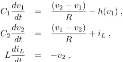
The Matsumoto-Chua circuit is a simple electronic circuit made of two capacitors, one linear resistor, one inductor, and one nonlinear diode (see Figs. 1(a) and 1(b)). This circuit is modeled by the equations

C1dv1

dt =

(v2−v1)

R −h(v1),

C2

dv2

dt =

(v1−v2)

R +iL, (1)

LdiL

dt = −v2,

whereC1andC2are the capacitors,v1andv2the tensions across the capacitors C1 andC2, R is the linear resistor,

L is the inductor, iL is the current across the inductorL,

andh(v1)is the characteristic curve in the (nonlinear) diode. The functionh(v1)(see Fig. 1(b)) is given by

h(v1) =m1v1+1

2(m2−m1)(|v1+BP|−|v1−BP|), (2) wherem1,m2, andBP are constants. We fixed the

follow-ing values for these parameters: 1/C1 = 9.0,1/C2 = 1.0,

1/L= 7.0,m1 =−0.5,m2=−0.8andBP = 1.0;Rthe

control parameter of the model.

2

C _v

2

iL

N_R i

R

v₁ C1

R

L

N_R

i

NR

V

m2

m1

(a) (b)

Figure 1. (a)Chua’s circuit, with two capacitors (C₁_andC₂_{), one}

linear resistor (R_{), one linear inductor (}L_{), and a nonlinear diode}

(Nr). (b) Characteristic curve of the non-linear diode.

(2)

been explored extensively in previous works (see for exam-ple [8]). For R ≈ 1.55, we can identify a symmetric pair of spiral-like attractors that, after a frontier crisis that oc-curs forR≈1.47, merge into a single attractor called by us “double-scroll”. In this work we analyze in detail the pair of spiral-like attractors for R = 1.510, R = 1.500, and

R = 1.495, which we callA,B, andC, respectively. Be-cause the pair of attractors is symmetric, only one of them needed to be analyzed. The results for attractorsA,B, and

C, are then compared with results obtained for a forth

attrac-tor,D, that appears for a slightly larger value ofR= 1.488, right after what may be the the onset of a hyperbolic regime. All the attractors were obtained from numerical integra-tion of equaintegra-tions 1. As an example, a picture of attractorB

can be seen in figure 2(a), together with its first return map (fig. 2(b)). AttractorsA,B andCshow a similar behavior. AttractorDwill be better discussed in section 4.

In order to build the first return maps, we used a Poincar´e sectionP_v+

1 defined by ⌋

P_v+ 1 =

(v1, v2, iL)∈R3|v1=v1+=

m2−m1

1/R+m1

, v2< v+2 = 0

, (3)

⌈

v

(a)

1 v2

0 1

(b)

w(i) w(i+1)

-0.6 -0.4 -0.2 0.0 0.2 0.4 0.6

-0.5 0.0 0.5 1.0 1.5 2.0 2.5 3.0 1.4 1.6 1.8 2.0 2.2 2.4 2.6

1.4 1.6 1.8 2.0 2.2 2.4 2.6

Figure 2. (a) Spiral-like attractorB, (R= 1.500_{), obtained from}

numerical integration of eq. (1). The full vertical line indicates the Poincar´e sectionP

v+

1 from which the first return map (b) was

obtained. AttractorsA_andC_{present a similar behavior.}

where(v₁+ = m2−m1 1/R+m1

,v₂+ = 0,i+_L =−v₁+)define one of the fixed points of the attractor. Following [9], and tak-ing advantage of the equivariant symmetry presented by the model, we adopted, for the first return map, a new variable

w=|iL|+ǫ|v2|, whereǫis an empirical factor (ǫ= 1.3for

attractorsA,B,C, and1.2for attractorD). If the first return map is written in terms of either iLorv2, the branches are

shown in duplicate, which makes it more difficult to identify the critical points and, consequently, establish the correct partition needed to code the dynamics. In Fig. 2(b) we see that, for attractor B, the first return map has two branches and a single critical point (atw=wc), as an unimodal map.

As usual, we associate the symbol 0with the left branch (w < wc) and the symbol1with the right branch (w > wc).

We observe essentially the same scenario for attractors A

andC. However, that does not happen for attractorD(see Fig. 4(d)). Now the first return map is bimodal, and we will need three symbols to code the dynamics.

3 Unstable periodic orbits and

sym-bolic dynamics

We combined two numerical methods to extract the unstable periodic orbits from attractorsA,B,CandD[9]. First, we estimate the positions of the unstable periodic orbits with a method known as close returns [10]. We then refined the estimate employing a Newton-Raphson algorithm, adapted to differential equations [11]. Each periodic orbit can then be identified by a (finite) sequence of pointsw(i), that are the intersections of the orbit with a Poincar´e section (in our case defined by (3)). The sequence of pointsw(i) is then codified into a symbolic sequenceSiof zeros and ones,

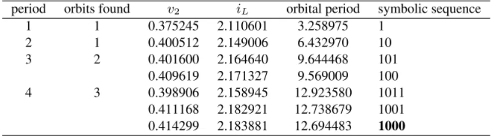
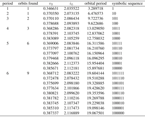
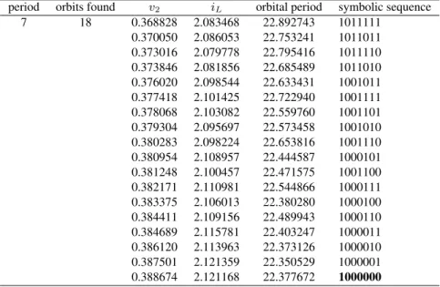
fol-lowing the usual procedure [7, 4, 5]. The results of applying this procedure to attractorsA,BandCare shown in tables I, II and III, respectively. In the tables, for each orbit, one can see the coordinatesiLandv2of the intersections of the orbit

with the Poincar´e sectionP_v+

1, its period, and the symbolic sequence that represents it.

TABLE I. Spectrum of unstable periodic orbits for attractorA_{up to period 4. For each orbit the table shows the period, the total number}

of orbits with the same period, coordinatesv₂andiL, orbital period and symbolic sequence. Coordinatesv2aniLare the coordinates of the (negative) periodic point farthest in the Poincar´e sectionP

v+

1

. The orbit codified by the symbol0is pruned and does not appear in the attractor.

period orbits found v₂ iL orbital period symbolic sequence 1 1 0.375245 2.110601 3.258975 1

2 1 0.400512 2.149006 6.432970 10 3 2 0.401600 2.164640 9.644468 101

0.409619 2.171327 9.569009 100 4 3 0.398906 2.158945 12.923580 1011

(3)

TABLE II. Spectrum of unstable periodic orbits for attractorB_{up to period 6. For each orbit the table shows the period, the total number}

of orbits with the same period, coordinatesv₂_andiL, orbital period and symbolic sequence. Coordinatesv₂aniLare the coordinates of the (negative) periodic point farthest in the Poincar´e sectionP

v+

1. The orbit codified by the symbol0is pruned and does not appear in the

attractor.

2 1 0.380220 2.098244 6.461487 10 3 2 0.380330 2.112240 9.696066 101

0.388819 2.119516 9.603776 100 4 3 0.378275 2.107688 12.992824 1011

0.388977 2.129868 12.804077 1001 0.393345 2.131243 12.734498 1000 5 6 0.379110 2.109425 16.264183 10111

0.383923 2.107424 16.170103 10110 0.387477 2.126501 16.109447 10011 0.389686 2.122016 16.062037 10010 0.393488 2.138606 15.911679 10001 0.395959 2.138435 15.866200 10000 6 9 0.378759 2.108697 19.546526 101111

0.382473 2.103817 19.459271 101110 0.385952 2.123788 19.283093 100101 0.388119 2.127780 19.375027 100111 0.391105 2.125702 19.309144 100110 0.392440 2.136122 19.220406 100011 0.394071 2.133682 19.189325 100010 0.396380 2.143670 19.036973 100001 0.397506 2.143324 19.018181 100000

TABLE III. Spectrum of unstable periodic orbits for attractorCup to period 7. For each orbit the table shows the period, the total number of orbits with the same period, coordinatesv₂andiL, orbital period and symbolic sequence. Coordinatesv₂aniLare the coordinates of the (negative) periodic point farthest in the Poincar´e sectionP

v+

1. The orbit codified by the symbol0is pruned and does not appear in the

attractor.

2 1 0.370350 2.073135 6.476573 10 3 2 0.370110 2.086434 9.722736 101

0.378688 2.093893 9.622686 100 4 3 0.368286 2.082318 13.029050 1011

0.378391 2.103745 12.837062 1001 0.383089 2.105259 12.758032 1000 5 6 0.369006 2.083846 16.311586 10111

0.373797 2.081734 16.210760 10110 0.377097 2.100762 16.150964 10011 0.379468 2.096118 16.096295 10010 0.382666 2.112373 15.954404 10001 0.385671 2.112181 15.897681 10000 6 9 0.368712 2.083222 19.604144 101111

(4)

Continuation.

0.370050 2.086053 22.753241 1011011 0.373016 2.079778 22.795416 1011110 0.373846 2.081856 22.685489 1011010 0.376020 2.098544 22.633431 1001011 0.377418 2.101425 22.722940 1001111 0.378068 2.103082 22.559760 1001101 0.379304 2.095697 22.573458 1001010 0.380283 2.098224 22.653816 1001110 0.380954 2.108957 22.444587 1000101 0.381248 2.100457 22.471575 1001100 0.382171 2.110981 22.544866 1000111 0.383375 2.106013 22.380280 1000100 0.384411 2.109156 22.489943 1000110 0.384689 2.115781 22.403247 1000011 0.386120 2.113963 22.373126 1000010 0.387501 2.121359 22.350529 1000001 0.388674 2.121168 22.377672 1000000

The dynamics of the system, in cases where it can be coded by two symbols only (unimodal maps), can be rep-resented by a diagram known as the alternating binary tree (see Fig. 3). The alternating binary tree represents all se-quences that form the itinerary; they appear in a specific order, known as “natural order” [11]. A given orbit is rep-resented by the specific sequence - among all compatibles with its itinerary - that appears most at right in the alternat-ing binary tree. It can be proved that, for unimodal maps [12], if an specific orbit is present in a dynamical system, all the other orbits that precede it according to the natural order will also be present. An inspection of Fig. 3 shows that, periodic orbits of periodn, represented by sequences of the forms(_hn) = (100...0)

n

(one followed by(n−1)zeros) are always at the extreme right of the binary tree. So, the iden-tification of an orbit of the types(_hn)means that the system has all possible orbits, up to leveln.

. .

.

. .

.

. .

.

. .

.

. .

. . .

.

. .

s_h(n)= 100...0 nível 3

nível 1

nível 2

nível n

00 01 11 10

000 001 011 010 110 111 101 100

0 1

level n level 3 level 2 level 1

Figure 3. Alternating binary tree for unimodal maps. In this di-agram the periodic orbits are ordered in a natural sequence, from left to right. If a periodic orbit is present in the attractor, all other orbits that precede it in this tree are also present.

An orbit predicted by the alternating binary tree, but not found in the dynamical system, is said to have been “pruned”. Note that, in the case of attractorA, some orbits start to be pruned forn= 5(see table I). The same behavior can be observed in attractorsB andC. But in those cases orbits start to be pruned forn= 7, andn= 8, respectively (see tables II and III). Note that the period 1orbit repre-sented by the symbolic sequence0is not present in any of the attractors.

In one-dimensional maps, as a dynamical system ap-proaches homoclinicity, that is, as the unstable manifold

Wu_{, associated with a saddle cycle or a saddle point}

ap-proaches and touches a stable manifoldWs_{, many}

homo-clinic points are created. As a consequence, the dynamics of the system becomes more and more complex, with more and more unstable periodic orbits. After the last tangency be-tween manifoldsWu_and_Ws_{, there is an infinite number of}

homoclinic points. When the homoclinic orbit appears, the dynamics reaches its highest degree of complexity; all pos-sible periodic orbits are present and the alternating binary tree is complete. We then say that the system has reached the hyperbolic regime.

A homoclinic orbit can be represented by the symbolic sequence OH = 1000... = snh→∞ = (100...) [2]. The

(5)

their chaotic behavior associated with the presence of a ho-moclinic orbit. In such cases the system is said to display homoclinic chaos. The analysis of those dynamical systems has been based on the identification of homoclinic bifurca-tions [3] - a sequence of saddle-node bifurcabifurca-tions that alter-nates with period-doubling bifurcations - that leads to the appearance of a homoclinic orbit. The occurrence of such a sequence of bifurcations, before the observation of a ho-moclinic orbit, has many times been considered sufficient to assume homoclinicity. This sequence induces a ramified structure in first-return maps, builded in a special way so they can capture the number of turns that a trajectory per-forms around a saddle point (or an unstable hyperbolic sad-dle cycle [2, 3]) before being reinjected in the attractor. Each of the branches of the first-return maps is associated with a specific number of turns that the system gives around the unstable saddle point or cycle.

The extrapolation, for smaller values of the control pa-rameterR, of the sequence of unstable periodic orbits found in attractors A, B andC (and shown, respectively, in ta-bles I, II and III), allows us to conjecture about the existence of a homoclinic orbitOH. This is better seen in table IV, which shows, for attractorsA,BandC, the last levelnfor which all sequences predicted by the alternating binary tree have been found. One can observe that the last sequence in the alternating binary tree is, up to some leveln, of the forms(_hn) = (100...0)

n

, with increasing values ofnfor de-creasing values ofR. The increase in the number of zeros in the orbits of table IV is associated with an increase in the divergent movement around the saddle cycle, in a typical be-havior of systems with a homoclinic orbit. This observation gives support to a conjecture that, in the Matsumoto-Chua circuit, as the parameterRdecreases, new orbits of period

n s(_hn) = (100...0) are created, filling up every level of the binary tree until the hyperbolic regime is attained. The analysis of the symbolic planes and fragmentation patterns gives further support to this conjecture.

TABLE IV. Last level (and the corresponding symbolic sequence) that presents a complete spectrum of orbits in the alternating binary tree, for attractorsA,BandC.

attractor R leveln s(_hn)

A 1.510 4 (1000) B 1.500 6 (100000) C 1.495 7 (1000000)

4 Symbolic planes

The changes in the dynamics introduced by the development of chaos in the Matsumoto-Chua circuit can be observed both in the first-return maps and in the symbolic planes, for attractorsA,B,C, andD.

The symbolic plane gives a way of summarizing the or-dering of symbolic sequences in a two-dimensional map. This method has been widely employed to identify topolog-ically similar systems (see examples in references [13], [15] and [14]). Each point(α, β)in a Cartesian plane is associ-ated with a possible sequence in a way described below. If all possible orbits are present, the plane is completely filled. Empty points, represent orbits that have been pruned and are forbidden. From the symbolic plane it is possible to identify the pruning fronts and the kneading sequences.

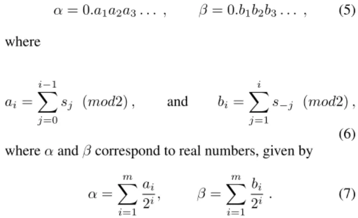
The coordinates(α, β)of a specific orbit or trajectory is built in a unique way from the symbolic sequence of ze-ros and ones that represents the orbit, through the following procedure. Let the symbolic sequence

. . . s−m. . . s−2s−1s0s1s2. . . sm. . . si∈0,1, (4)

represent a given trajectory. The symbols0(representing the current position of the system) splits the sequence into two parts, a forward sequence given bys0s1s2. . . sm. . . which

represents the “symbolic future”, and a backward sequence

. . . s−m. . . s−2s−1, which represents the “symbolic past”. The symbolic coordinates(α, β)for the point that will rep-resent this orbit are then given, in binary notation, by

α= 0.a1a2a3. . . , β = 0.b1b2b3. . . , (5) where

ai=

i−1

j=0

sj (mod2), and bi=

i

j=1

s−j (mod2),

(6) whereαandβcorrespond to real numbers, given by

α=

m

i=1

ai

2i, β= m

i=1

bi

2i . (7)

This formalism can be extended to represent a dynamics described by3or more symbols (see, for example,[15] and [16]).

In Figs. 4(a), 4(b), 4(c) and 4(d) we can see the first re-turn maps and the symbolic planes for attractors A,B, C

andD, respectively. The first return maps of attractorsA,

BandCshow that those attractors have a unimodal behav-ior, and can essentially be described by a symbolic dynamics made of two symbols. The first-return map for attractorA

(R= 1.510) indicates that the system does not have all pos-sible orbits; the symbolic plane shows many forbidden re-gions (empty rere-gions) together with allowed rere-gions (filled with dots). Comparing with Figs. 4(b) and 4(c) (attractors

(6)

(c)

0 1

1 0

(d)

0 1 2

0 1

w(i+1) β

α

w(i)

(B) (A)

(C)

(D) (a)

(b)

1.4 1.6 1.8 2.0 2.2 2.4 2.6 1.4

1.6 1.8 2.0 2.2 2.4 2.6

0.4 0.6

0.2 0.8

0.6 0.4 0.2

0.0 0.8 1.00.0

1.0

Figure 4. First-return maps and corresponding symbolic planes for attractorsA,B,C andDrespectively. We can observe that, as the parameterRdecreases, the symbolic plane is more and more complete. FromAtoCthe symbolic planes show an increase in the allowed regions, indicating the approach of the hyperbolic regime. AttractorDshows a complete different scenario. The first-return map is not unimodal anymore, and in the symbolic plane (now associated with a symbolic dynamics of three symbols) we observe a predominance of forbidden regions.

Figure 4(d) (attractorD, withR= 1.488) shows a com-pletely different scenario, with the drastic changes in the behavior of the system that may have been induced by the onset of a homoclinic regime. Now the first-return map is bimodal. The symbolic plane, now built with a dynamics of three symbols, is completely different, with many forbidden regions.

In unimodal maps with a unidimensional structure, the pruning front, in the symbolic plane, is a continuous line, while in two-dimensional maps the pruning front is discon-tinuous [14]. Fig. 5, an amplification of the symbolic planes presented in Fig. 4, clearly shows that there is a disconti-nuity in the pruning fronts of attractorsA,B andC, indi-cating that they do have a two-dimensional structure. We

see, however, that those pruning fronts get closer and closer to each other as we go from attractor A to C 1_{. In}

or-der to measure how good is the one-dimensional approxi-mation, we can define an indexd, equal to the integer part oflog₂( 1

α2−α1), whereα1andα2define the smaller and

larger pruning fronts, respectively. The indexd gives the level, in the binary tree, up to which the behavior of the sys-tem can be considered one-dimensional. For instance, for attractor A, α1 = 0.9472 andα2 = 0.9605, sodA = 4.

Analogously, dB = 7 anddC = 11. Those results show

that the one-dimensional approximation becomes better and better as the chaotic regime evolves.

(7)

(c)

β

α

(b)

α β

(a)

α β

0 0.1 0.2 0.3 0.4 0.5 0.6 0.7 0.8 0.9

1

0.991930 0.992415 0 0.1 0.2 0.3 0.4 0.5 0.6 0.7 0.8 0.9 1

0.98245 0.98805 0

0.1 0.2 0.4 0.5 0.6 0.7 0.8 0.9 1

0.9605 0.9472

0.9615 0.3

Figure 5. Blow up of the pruning front region of Figs. 4A, 4B and 4C, showing the two-dimensional structure of attractorsA_,B_and C.

We are aware that, if we have a 2D map, the existence of a10n_{orbit does not force the existence of all previous orbits}

of the natural sequence, as it happens in 1D maps. How-ever, we think that we have strong indications that, at least in these case, as the chaotic regime evolves and the dynam-ics of the system becomes more and more one-dimensional, it approaches the dynamical behavior of a typical unimodal map, and our observations may in fact indicate the existence of homoclinic chaos. It would be interesting to observe if, in other systems, for which it is well established that the hy-perbolic regime is reached, the same scenario is found.

The fragmentation patterns (see Fig. 6) give another way of showing that Chua’s circuit may be approaching a homo-clinic regime. Through those patterns one can build a picto-rial representations of the symbolic sequences that represent the trajectories. We associate a black block with symbol1 and a white block with symbol0. For instance, the sequence 100would be represented by the sequence of blocks “black-white-white”. The blocks are placed in sequence, side by side, from left to right, up to 50 blocks; after that, a new row of symbols is added on top of the previous one. The process continues until a grid of50×50 blocks is built. As the chaotic regime evolves, the allowed trajectories will present an increasing number of symbols0, associated with the di-vergent movement around the saddle cycle, as compared to the number of symbols“1”, associated with the reinjection movement.

(b) (a)

(c)

Figure 6. Fragmentation patterns for symbolic sequences of attrac-torsA,BandCrespectively.

By visual inspection, it is possible to see that the orbits of attractor A(Fig. 6a) have a predominance of symbols1

(black blocks), while in attractorC(Fig. 6c) there is a pre-dominance of symbols0, reflecting the fact that, as the pa-rameterRdecreases, the trajectories stay longer and longer in a divergent movement around the saddle cycle.

5 Conclusions

In conclusion, we have extracted the unstable periodic orbits from attractorsA,B,CandDof the Matsumoto-Chua cir-cuit. We have used symbolic dynamics in order to show that as the chaotic regime evolves the Matsumoto-Chua circuit has a dynamics that is increasing one-dimensional. We have presented numerical evidence that a homoclinic orbit may be present in the Matsumoto-Chua circuit. The attractors of the dynamics of the circuit were analyzed for four different values of the control parameterR,R∈[1.510,1.4888]. We found that there is a pattern in the way new unstable periodic orbits are created as the control parameterRis continuously decreased. From this pattern, if the system had a truly 1D dynamics, it would be possible to infer the existence of a homoclinic orbit. If this behavior comes to be checked in similar systems, it will be a new approach to the problem of identifying the onset of homoclinicity that could be used in many other problems, either in experimental situations or numerical simulations.

For each of the studied attractors (attractorsA, B and

C), we have extracted the unstable periodic orbits, built first-return maps, codified the dynamics and ordered the or-bits according to the natural order in an alternating binary tree. It has been possible to see that the last orbit in the di-agram, before orbits start to be pruned, was always of the form s(n) _{= (100}_...₀₎

n

, with n → ∞ as the parameter R

(8)

as in a one-dimensional map, until the hyperbolic regime is attained. We conjecture that, because the behavior of the system becomes close to a one-dimensional map, maybe a homoclinic orbit exists in this circuit.

We also built symbolic planes and fragmentation pat-terns for all the studied sequences and trajectories, which gives further support to our conjecture.

6 Acknowledgements

We acknowledge the financial support of the Brazilian agency CNPq.

References

[1] P. Gaspard, R. Kapral, G. Nicolis, J. Stat. Phys. 35, 697 (1984).

[2] T. Braun, J. A. Lisboa, Int. J. Bifurc. Chaos,4, 1483 (1994).

[3] F. Papoff, A. Fioretti, E. Arimondo, Phys. Rev. A44, 4639 (1991).

[4] J. Plumecoq, M. Lefranc, Physica D144, 231 (2000).

[5] N. B. Tufillaro, T. Abbott, J. Reilly, An experimental ap-proach to nonlinear dyanamics and chaos(Addison-Wesley, California, 1992).

[6] W. M. Gonc¸alves, R. D. Pinto, J. C. Sartorelli, Physica D134, 267 (1999).

[7] J. Milnor and W. Thurston, in Dynamical Systems, ed. J. Alexander, Lecture Notes in Math.1342, spring-Verlag, Berlin, (1988).

[8] R. N. Madan,Chua’s circuit: a paradigm for chaos, (World Scientific, Singapore, 1993).

[9] C. Letellier, P. Dutertre, G. Gouesbet, Phys. Rev. E49, 3492 (1994).

[10] D. P. Lathrop, E. J. Kostelich, Phys. Rev. A40, 4028 (1989); G. B. Mindlin, Gilmore, Physica D58, 229 (1992).

[11] B. -L. Hao,Elementary Symbolic Dynamics and Chaos in Dissipative Systems, (World Scientific, Singapore, 1984). [12] P. Glendinning, C. Laing, Phys. Letters A211, 155 (1996); S.

V. Gonchenko, L. P. Shilnikov and D. V. Turaev, Chaos6, 15 (1996); R. L. Devaney,An introduction to chaotic dynamical systems, (Addison-Wesley, second ed., Boston 1988). [13] A. Tufaile, J. C. Sartorelli, Phys. Lett. A275, 211 (2000).

[14] P. Civitanovi´c, G. H. Gunaratne and I. Procaccia, Phys. Rev. A38, 1503 (1988).

[15] C. Letellier, G. Gouesbet and N. F. Rulkov, Int. J. Bifurc. Chaos6, 2531 (1996).