Image Gradient Applied to
Morphological Segmentation
Franklin C´esar Flores
1,2, Airton Marco Polid´orio
1& Roberto de Alencar Lotufo
21Department of Informatics
State University of Maring´a Av. Colombo, 5790, Zona 7 Phone: +55 (44) 32635874 (FAX) Zip 13081-970 - Maring´a - PR - BRAZIL
{fcflores — ampolido}@din.uem.br
2
Department of Computer Engineering and Industrial Automation School of Electrical and Computing Engineering
State University of Campinas
P.O.Box 6101, Zip 13083-852 - Campinas - SP - BRAZIL
{fcflores — lotufo}@dca.fee.unicamp.br
Abstract
This paper proposes a method for color gradient com-putation applied to morphological segmentation of color images. The weighted gradient (with weights estimated automatically), proposed in this paper, applied in con-junction with the watershed from markers technique, pro-vides excelent segmentation results, according to a sub-jective visual criterion. The weighted gradient is com-puted by linear combination of the gradients from each band of an image under the IHS color space model. The weights to each gradient are estimated by a systematic method that computes the similarity between the image to compute the gradient and an ”ideal image”, whose his-togram has an uniform distribution. Several experiments were done in order to compare the segmentation results provided by the weighted gradient to the results provided by other color space metrics, also according to a sub-jective criterion, and such comparison is present in this paper.
Keywords:Weighted Gradient, Color Gradient, Mor-phological Segmentation, Watershed from Markers, Bray-Curtis Distance Function, Weight Estimation
1. Introduction
The edge enhancement of an image by gradient com-putation is an important step in morphological image segmentation via watershed from markers [1, 10]. For
grayscale images, the morphological gradient [14, 7] is a very good option and its computation is simple: for each point in the image, a structuring element is centered to it and the difference between the maximum and the min-imum graylevels inside the structuring element is com-puted. Here, the similarity information exploited is the intensity differences among pixels inside the structuring element.
Such concept does not extends naturally to color im-ages. Despite the similarity information of color images is richer than the similarity of grayscale ones, the design of methods to edge enhancement in color images is complex. Note that the metric that measures the natural similarity information of color images is unknown. Also note that if one considers the color space as a complet lattice [15, 2], the order relation is not total and even if a total order is imposed, it will be not natural for the human eye. It does not compare two colors and decides which one is higher. It makes no sense to say: ”yellow is higher than blue”.
infor-mation contained in a band, the greater the weight to be assigned to its gradient. For instance, if the color image presents a great variation of hues, the hue gradient should receive a major weight.
One way to compute automatically the weights to each band is via application of a similarity function [3]. The idea is to consider an ”ideal image” (whose histogram has a uniform distribution) and to compute the similarity be-tween the input image and the ideal one. Several ways to compute the similarity between pairs of objects (in our case, images) were found in the literature [13, 5, 9]. In this paper, the similarity is computed by a distance func-tion calledBray-Curtis distance[13] which gives a value from 0 (similarity) to 1 (not similarity). The weight to a gradient is given by the application of this distance func-tion.
This paper is organized as follows: section 2 presents preliminary definitions. Section 3 gives the definitions of weighted gradient. Section 4 states the Bray-Curtis dis-tance function, used to estimate the weights. Section 5 in-troduces the weight estimator to the weighted gradient op-erator. Section 6 explains the morphological image seg-mentation via watershed form markers. Section 7 shows the comparison among several color image gradients and the segmentation results provided by them. And, finally, we conclude this paper in section 8.
2. Preliminary Definitions
This section presents some definitions used along the text.
2.1. Color Images
Apartial ordered relationis a relation whose prop-erties is reflexive, transitive and anti-symmetric. A set whose elements have partial order relation is called a par-tial ordered set. Given a ordered setL, with a relation order ”≤”.Lis atotally ordered setif,∀x, y∈L,x≤y ory ≤x. The relation order ”≤” is saidtotal. A partial ordered set Lis acomplete lattice (also calledchain) if any subset ofLhave an infimum and a supremum.
LetL1, L2,· · ·, Lm be totally ordered complete
lat-tices. For instance: a subset ofZ, or a closed subset ofR are chains. LetWdenote thesupremum, or maximum, and V
denote theinfimum, or minimum, operations in chains. Let Lbe the Cartesian product of L1, L2,· · ·, Lm, i.e.,
l∈L⇔l={l1, l2,· · ·, lm}, li ∈Li, i={1,· · ·, m}.
LetEbe a non empty set that is an Abelian group with respect to a binary operation denoted by+. A mapping f fromE toL, f(z) = (f1(z), f2(z),· · ·, fm(z)),fi :
E→Liandz∈Eis calledmultivaluedormultispectral
image. The mappingsfi are calledbandsof the image.
A color image is an example of a multivalued function whereL=L1×L2×L3is the representation of the colors under a certain color space model (a coordinate system where each point represents an unique color) [6, 11]. Let
F un[E, L] denote the set of all mappings fromE toL, i.e., all possible color images.
2.2. Color Space Models
In this paper, we used two color space models: the RGB (Red,GreenandBlue) and the IHS (Intensity,Hue andSaturation) color coordinate systems.
The RGB color space model is a cube defined in a Cartesian system. This cube is defined by three subspaces related to one of the three primary colors,red,greenand blue, and the pure representation of these colors are lo-cated at three corners of the cube. Generally, one color is represented by a point inside this cube.
The IHS color space model is defined by a coordinate transformation of the RGB system [11], and it is com-posed by three attributes: Intensity(holds the luminosity information),Hue(describes uniquely a color in its pure form); for example, the red color without any informa-tion from other attributes) and Saturation(measures the amount of white light mixed with pure colors).
3. Weighted Gradient
In this section, we present the definition of the weighted gradient. This operator is a transformation from a color image under the IHS color space to a grayscale one, by the linear combination of the gradients from each band.
LetK = [0,1,· · ·, k−1]andΘ = [0,359]. The setK is a closed interval and has a total order relation. The set Θ, however, does not have such relation, since it can be considered as a ”circular interval”, because its elements are angles [6]. Let f ∈ F un[E, L]be a color image under the IHS color space model, whereE ⊂Z×Z andL=K×Θ×K.
Since intensity and saturation are represented by func-tionsg∈F un[E, K], their gradients can be computed by classical morphological gradient operators [14, 7]. How-ever, it is not the case for hue: since the information of the hue band consists of angles [6], the band is given by a functionh ∈ F un[E,Θ], and its gradient can not be computed by classical morphological gradient, becauseΘ does not have a total order relation. In order to compute a gradient for the hue band, it is necessary to define a metric function for it.
Definition 3.1 Letθ1, θ2∈Θ. The hue distance between θ1andθ2is given by
dh(θ1, θ2) =∧{|θ1−θ2|,360− |θ1−θ2|}.
The distance introduced above returns an integer value between 0 and 180. In order to compute the weighted gradient, these values will be normalized toK. LetmK:
Θ→Kbe the normalization function.
Definition 3.2 Given an imageh∈ F un[E,Θ], the an-gular gradient∇Θ
B :F un[E,Θ]→F un[E, K], is given
by, for allx∈E
∇Θ
B(h)(x) =mK(
W
y∈{Bx−{x}}dh(h(x), h(y)) −Vy∈{Bx−{x}}dh(h(x), h(y))),
where B ⊂ E is a structuring element centered at the origin ofE.
Leta, b, c∈R+. The following gradient is defined as a linear combination of the morphological gradients for the intensity and saturation bands with the angular gradi-ent for the hue band. The three gradigradi-ents are weighted by three weightsa,bandcin order to enhance or to obscure the peaks of a gradient image.
Definition 3.3 Given f ∈ F un[E, L] in the IHS color space. Given three weight values a, b, c ∈ R+. The weighted gradient ∇W
B : F un[E, L] → F un[E,Z+] is
defined by
∇W
B(f) =⌊a∇B(f1) +b∇ΘB(f2) +c∇B(f3)⌋,
wheref1,f2and f3 represent respectively the intensity, hue and saturation color bands, B ⊂ E is a structur-ing element centered at the origin of E and ∇B is the
classical morphological gradient [14, 7]. The floor oper-ation in the equoper-ation means that all∇W
B(f)(x),x∈ E,
were rounded down, since the linear combination of the weighted gradients is real.
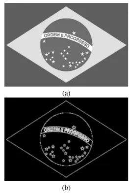
In the weighted gradient, each gradient is scaled in order to increase or decrease their influence in the final result. For example, on images where the hue informa-tion is the most important, the hue gradient could give a good result by itself. However, there are cases that it is not sufficient to enhance the border between objects with similar hues; it could be necessary to weight, for example, the saturation gradient in order to distinguish the borders. Figure 1 (b) shows the result of the weighted gradient applied to Fig. 1 (a). The weights assigned to the hue, saturation and intensity gradients are, respectively, a = 0.1055,b= 0.1016andc= 0.1133.
The first version of the weighted gradient operator was introduced in [8]. Despite this operator shows itself as a good solution to compute color gradients, it was not defined, in that occasion, a systematic method to find weights to each gradient: the weights assigned to each gradient in the linear combination step had been imposed manually. It was necessary a priori to analyze subjec-tively the color image to be segmented in order to choose the weights to be applied. Sometimes, it was necessary to readjust several times the weights to achieve a satisfac-tory result. It motivated the design of the weight estimator presented in section 4 and the automatic weighted gradi-ent introduced in section 5.
(a)
(b)
Figure 1. Weighted Gradient - (a) Original Image. (b) Gradient.
4. Bray-Curtis Distance Function
A similarity function quantifies the association degree between a pair of objects. We have found that similarity functions could be suitable for application in order to esti-mate the weights to the gradients [13, 5, 9]. In the method introduced below, it was used a well known method to numerical ecology researchers, the Bray-Curtis distance function [13]. The distance measured by this function gives a degree of similarity, which is a value from 0 to 1. The closer the degree is to 0 (1), the greater (lower) the similarity. The Bray-Curtis distance function is defined below.
Definition 4.1 Let Aand B be twon-dimensional vec-tors. The Bray-Curtis distance functionD : A×B →
[0,1], is given by,
D(A, B) = Pn
i=1|Ai−Bi|
Pn
i=1(Ai+Bi) ,
whereAi andBiare, respectively, thei-th element ofA
and thei-th element ofB.
5. Weight Estimation
1. if there are many different hues appearing in the im-age, it is imposed a high weight to the hue gradient original;
2. if there are just blue tones in the image, the hue gra-dient is not so important and its weight could be low (however, this gradient does not need to be dis-carded, since it can still help to separate, for exam-ple, objects with similar saturation);
3. if the image presents a great variation in luminance, the intensity gradient should receive a higher weight.
Despite the drawback of manual imposition of weights, the weighted gradient gives excellent results when the criterion cited above is applied. This criterion also should be applied to the automatic method to weight estimation in order to still achieve good results.
If a band presents all possible values in same quan-tities (i.e., its histogram has an uniform distribution), its gradient should receive the maximum weight. To do this, we consider that there is an ”ideal image” where all possi-ble values appear in same quantities (i.e., with a histogram whose distribution is an uniform one). The distance be-tween the band and the ideal image is computed; if the distance is closer to 0, it means that the information in the band is rich and the weight to be assigned should be high. The distance between the band and the ideal image can be obtained by computing the distance between their histograms. Note that there is no real ”ideal image” but just only its histogram, which has an uniform distribution. Such histogram is easy to be created: just consider it as a function with constant value equals to the mean of his-togram of the band.
Definition 5.1 Let us consider the histogram of an image f ∈ F un[E, K]as a functionhf : K → Z+. Letfi :
E → Li be one of the image bands and letgi : E →
Li be the ideal image. The weight wi assigned to the
gradient offiis given by,
wi= 1−D(hfi, hgi),
whereD is the Bray-Curtis distance function andhgi is
the histogram of the ideal image, computed as explained above.
Bray-Curtis distance function is a simple and suitable way to compute the weight to a gradient. Its computation is fast and it gives the similarity measure as a normalized value contained in the interval [0,1](whose boundaries denotes, in our approach, respectively, similarity and dis-parity), and thus, providing a simple way to estimate the weight by the criterion pointed above.
Note that the Bray-Curtis distance function gives small results when the histograms are close to. So, it is necessary to subtract the function result from 1 (the max-imum weight possible) in order to obtain the weight to the gradient.
Given the definition above, the weighted gradient can be redefined as follows:
Definition 5.2 Given f ∈ F un[E, L] in the IHS color space. The weighted gradient ∇W
B : F un[E, L] →
F un[E,Z+]is defined by
∇W
B(f) =⌊w1∇B(f1) +w2∇ΘB(f2) +w3∇B(f3)⌋.
wheref1,f2and f3 represent respectively the intensity, hue and saturation color bands, w1, w2, w3 ∈ R+ are their respective weights estimated by the distance func-tion, B ⊂ E is a structuring element centered at the origin of E, ∇B is the classical morphological
gradi-ent [14, 7] and∇Θ
Bis the angular gradient.
In the following, it is presented some experiments done in order to demonstrate the estimation of weights by Bray-Curtis distance function. Each experiment con-sisted in a creation of a synthetic pure blue image under a IHS color space model and changing one of the bands by the classical cameraman image, in order to enrich the in-formation of the band and, thus, to demonstrate how the method assigns a higher weight to this band. The syn-thetical image created to the hue, saturation and intensity experiments are shown, respectively in Fig. 2 (a), 3 (a) and 4 (a).
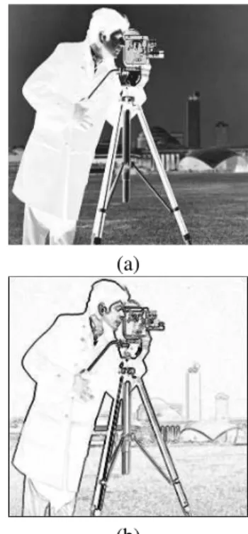
In the first experiment (Fig. 2), we demonstrate the estimation to the hue band. Figure 2 (a) shows an image obtained by taking a constant blue image and changing its hue band by the classical cameraman normalized im-age. We want to show that, since the hue band is the most important in this image (saturation and intensity bands in this image are constant), the weight to be assigned to the hue gradient should be high and the weights assigned to the saturation and intensity bands should be low.
The proposed distance function computed the follow-ing weights to Fig. 2 (a): huew1 = 0.8945, saturation w2 = 0.0039and intensityw3 = 0.0039. Figure 2 (b) shows the weighted gradient of Fig. 2 (a).
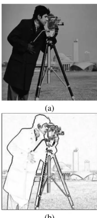
The other two experiments shown in this section are similar to the first one. Figure 3 (a) was obtained by tak-ing a constant blue image and changtak-ing its saturation band by the cameraman image. The saturation band of Fig. 3 (a) is the most important band, since the other two bands are constant, so it is expected that the weight assigned to the saturation gradient should be high and the other two weights should be low. The distance function provided to Fig. 3 (a) the weights: hue w1 = 0.0078, saturation w2 = 0.8555and intensityw3 = 0.0039. Figure 3 (b) shows the weighted gradient of Fig. 3 (a).
(a)
(b)
Figure 2. Hue - (a) Original Image. (b) Gradient.
6. Watershed from Markers
Morphological segmentation via watershed from markers [1] consists in a sequential application of mor-phological operators [7] to segment objects in the image. Basically, it consists in application of morphological gra-dient operator [7, 4], marker selection and watershed from markers technique [1, 16].
The watershed from markers can be described by flooding a topographical relief model of the gray-scale image. The markers are holes in the image relief where colored water can enter as the relief is flooded. There is one color associated to each set of markers. As the relief is uniformly flooded, different colored water may meet but cannot be mixed. When all the relief is flooded, each colored water region defines thecatchment basin[12] as-sociated to the marker. The classical watershed transform is when the markers are the regional minima of the image. Watershed from markers is an efficient method to im-age segmentation, since it reduces the problem of objects segmentation to the problem of finding markers to these objects.
7. Experimental Results
This section presents the segmentation results pro-vided by application of several color image gradients. All of them, excepting the automatic weighted gradient, pro-posed in this paper, were compared previously in [8] and the manual weighted gradient provided the best segmen-tation results. The experiments described below aim to compare the automatic and the manual weighted
gradi-(a)
(b)
Figure 3. Saturation - (a) Original Image. (b) Gradient.
ents to other gradients introduced in [8]. It is expected segmentation results provided by the automatic weighted gradient, at least, as good as the results provided by the manual method.
Preceding the experiment descriptions, it is necessary to review the gradients that will be compared. Note that the weighted gradient is applied to color images under the IHS color space model. The following operators (Gradi-entsItoIV) are applied to color images under the RGB color space model.
7.1. GradientI
Letf ∈ F un[E, L], the Gradient Iof f,∇I B(f)is
given by
∇IB(f) =
_
{∇B(f1),∇B(f2),∇B(f3)},
where∇B(f)is the morphological gradient. The
result-ing gradient is an image containresult-ing the supremum among the maxima differences em each band off.
7.2. GradientII
Letf ∈F un[E, L], the GradientII off,∇II B(f)is
given by
∇II B(f) =
_
{∇i B(f1),∇
i B(f2),∇
i B(f3)},
where ∇i
B(f) = f −εB(f)is the internal
(a)
(b)
Figure 4. Intensity - (a) Original Image. (b) Gradient.
7.3. GradientIII
LetdIII be thenormof a colorl∈L, given by
dIII(l) =⌊(l12+l22+l23)
1 2⌋,
where⌊p⌋is the value ofprounded down. Letax,B, bx,B ∈Eare two points such that
dIII(f(ax,B)) =
_
y∈Bx
dIII(f(y)),and
dIII(f(bx,B)) =
^
y∈Bx
dIII(f(y)).
Letf ∈F un[E, L], the GradientIII off,∇III B (f)
is given by
∇III
B (f)(x) =dIII(uf,x,B),
where uf,x,B = (f1(ax,B) − f1(bx,B), f2(ax,B) −
f2(bx,B),
f3(ax,B)−f3(bx,B)).
7.4. GradientIV
LetdIV be the color distance betweenlandl′,l, l′ ∈
L, given by,
dIV(l, l′) =
_
{|l1−l′1|,|l2−l2′|,|l3−l′3|}.
Letf ∈F un[E, L], the GradientIV off,∇IV B (f)is
given by
∇IVB (f)(x) =
_
y∈Bx
dIV(f(x), f(y)).
7.5. Segmentation Results
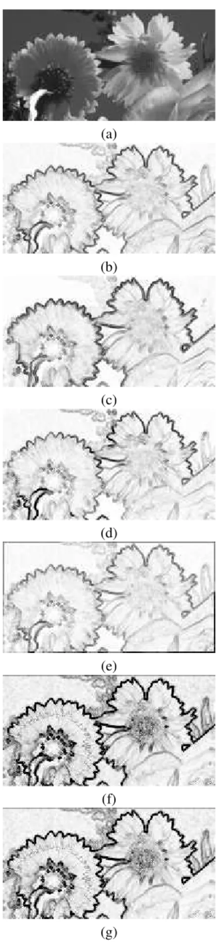
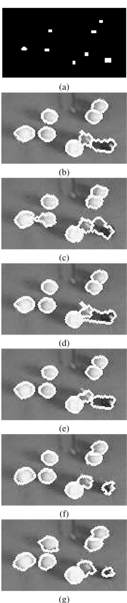
The first experiment consists in to segment the three flowers (Fig. 5 (a)) given the set of markers imposed man-ually to each flower and to the background (Fig. 6 (a)). Note the difficult in to distinguish the borders among the flowers, mainly between the middle and right ones. Here, the segmentation results were compared.
Figures 5 (b-e) show, respectively the results of Gra-dient I, II, III, IV. Figure 5 (f) shows the manual weighted gradient (with weights{a= 1, b= 1, c = 1}) and Fig. 5 (g) shows the automatic weighted gradient (whose estimated weights were {w1 = 0.9570, w2 = 0.9219, w3= 0.9336}). Figure 6 (b-g) show their respec-tive segmentation results. Again, in order to have a better visualization, the gradient images were negated and the watershed lines were dilated and overlaid to the original image.
All gradients provided the correct segmentation of the left flower, but the separation of the middle flower from the rightest one showed to be critical. GradientsItoIV segmented the middle flower with a piece of the rightest one. Both weighted gradients almost segmented correctly the flowers. Note that the contrast between the middle and the right flowers is very low.
The goal in the second experiment was to segment a set of billiard balls from the table (Fig. 7 (a)), given the set of markers shown in Fig. 8 (a), by application of the gra-dients presented above and to compare subjectively their segmentation results.
Figures 7 (b-e) show, respectively the results of Gra-dient I, II, III, IV. Figure 7 (f) shows the manual weighted gradient (with weights{a= 1, b= 1, c = 1}) and Fig. 7 (g) shows the automatic one (whose esti-mated weights were{w1 = 0.5977, w2 = 0.7109, w3 = 0.1055}). Figure 8 (b-g) show their respective segmen-tation results. The gradient images were negated and the watershed lines were dilated and overlaid to the original image for a better visualization.
GradientIprovided a good segmentation of the balls, except to the black one; this ball and its shadow were seg-mented together. The black ball segmentation showed it-self a critical problem since it was not also achieved by the GradientsII,III andIV. GradientII provides an un-pleasant segmentation of the ball and GradientsIII and IV did not achieved a good segment of the red ball.
Both manual and automatic weighted gradients pro-vided good segmentation results, excepting by a minor distortion in the segmentation of the pink ball, the seg-mentation results provided by the automatic method is very close to results provided by the manual one.
(a)
(b)
(c)
(d)
(e)
(f)
(g)
Figure 5. First Experiment -Flowers: (a) Original Image. (b-e) GradientsItoIV. (f) Manual Weighted Gradient. (g) Automatic Weighted Gradient
(a)
(b)
(c)
(d)
(e)
(f)
(g)
(a)
(b)
(c)
(d)
(e)
(f)
(g)
Figure 7. Second Experiment -Billiard Balls: (a) Origi-nal Image. (b-e) GradientsItoIV. (f) Manual Weighted Gradient. (g) Automatic Weighted Gradient
(a)
(b)
(c)
(d)
(e)
(f)
(g)
(a)
(b)
(c)
(d)
(e)
(f)
(g)
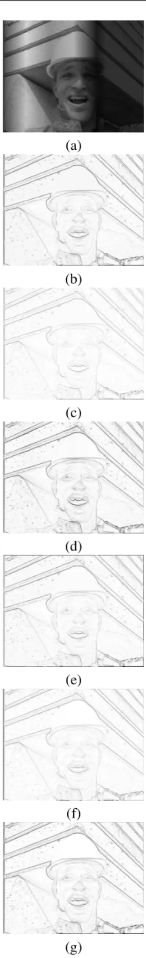
Figure 9. Third Experiment -Color Foreman: (a) Origi-nal Image. (b-e) GradientsItoIV. (f) Manual Weighted Gradient. (g) Automatic Weighted Gradient
(a)
(b)
(c)
(d)
(e)
(f)
(g)
given the set of markers in Fig. 10 (a). Again, the seg-mentation results are compared subjectively.
The results of GradientI,II,III,IV are shown, re-spectively, in Fig. 9 (b-e). Figure 9 (f) shows the manual weighted gradient (with weights{a= 1, b= 1, c = 1}) and Fig. 9 (g) shows the automatic one (whose esti-mated weights were{w1 = 0.7305, w2 = 0.0078, w3 = 0.9844}). Figure 10 (b-g) show their respective seg-mentation results. Once more, the gradient images were negated and the watershed lines were dilated and overlaid to the original image.
Note that the helmet region showed itself critical in the segmentation process. GradientsI,II,III andIV missed in several degrees the helmet border and the back-ground invaded the helmet. GradientIV also provided a wrong segmentation in the eye of the foreman.
The trivial set of weights imposed to the manual ver-sion of the weighted gradient ({a = 1, b = 1, c = 1}) did not provide a correct segmentation result. The top of the helmet joined to the upper background. The auto-matic weighted gradient estimated a better set of weights
{w1 = 0.7305, w2 = 0.0078, w3 = 0.9844}) and pro-vided a correct segmentation of the foreman.
8. Conclusion
This paper proposes a gradient for color images by linear combination of weighted gradients from the three bands of an image under the IHS color space model: the weighted gradient operator. The function of the weights is to raise or lower the contribution of each gradient in the linear combination, and they are estimated by an au-tomatic method that computes the similarity between the band histogram and an histogram whose distribution is uniform. Such similarity is computed by a Bray-Curtis distance function, whose gives a value from 0 (similarity) to 1 (not similarity).
Several experiments were done in order to compare the segmentation results provided by various color gradi-ents following a subjective visual criterion. The weighted gradient, with weights estimated by Bray-Curtis distance function, provided the best segmentation results.
One of the advantages of the proposed method is that it not requires any parameters other than the color image itself and a connectivity parameter. The evaluation crite-rion of the diversity of information in an image, given by the distance between the image band and an ”ideal im-age” whose histogram has an uniform distribution, is a very good criterion to give weights to each band gradi-ents.
Future works include the application of other tech-niques, such as other distance functions and information theory methods (as first-order entropy), in order to do weight estimation in the proposed framework. It will be also studied the exploitation of other color space models in order to compute color gradients.
9. Acknowledgements
The second author is on leave from UEM to UNESP at Presidente Prudente-SP-Brazil for doctorate purposes.
References
[1] S. Beucher and F. Meyer. Mathematical Morphol-ogy in Image Processing, chapter 12. The Morpho-logical Approach to Segmentation: The Watershed Transformation, pages 433–481. Marcel Dekker, 1992.
[2] J. Chanussot and P. Lambert. Total Ordering Based on Space Filling Curves for Multivalued Morphol-ogy. In Henk J.A.M. Heijmans and Jos B.T.M. Roerdink, editors, Mathematical Morphology and its Applications to Image and Signal Processing, volume 12 ofComputational Imaging and Vision, pages 51–58. Kluwer Academic Publishers, Dor-drecht, May 1998.
[3] F. C. Flores, A. M. Polid´orio and R. A. Lotufo. Color Image Gradients for Morphological Segmen-tation: The Weighted Gradient Improved by Auto-matic Imposition of Weights. In IEEE Proceed-ings of SIBGRAPI’2004, pages 146–153, Curitiba, Brazil, October 2004.
[4] F. C. Flores, R. Hirata Jr., J. Barrera, R. A. Lotufo, and F. Meyer. Morphological Operators for Segmen-tation of Color Sequences. InIEEE Proceedings of SIBGRAPI’2000, pages 300–307, Gramado, Brazil, October 2000.
[5] G. F. Estabrook, D. J. Rogers. A general method of taxonomic description for a computed similarity measure.Bioscience, 16:789–793, 1966.
[6] R. C. Gonzalez and R. E. Woods. Digital Image Processing. Addison-Wesley Publishing Company, 1992.
[7] H. J. A. M. Heijmans. Morphological Image Oper-ators. Academic Press, Boston, 1994.
[8] R. Hirata Jr., F. C. Flores, J. Barrera, R. A. Lotufo, and F. Meyer. Color Image Gradients for Morpho-logical Segmentation. InIEEE Proceedings of SIB-GRAPI’2000, pages 316–322, Gramado, Brazil, Oc-tober 2000.
[9] J. C. Gower. A general coeficient of similarity and some of its properties. Biometrics, 27:857–871, 1971.
[11] Pratt. Digital Image Processing, chapter 18. Image Segmentation, pages 597–627. Wiley, 1991.
[12] R. A. Lotufo and A. X. Falc˜ao. The Ordered Queue and the Optimality of the Watershed Approaches. In J. Goutsias, L. Vincent, and D. S. Bloomberg, edi-tors,Mathematical Morphology and its Applications to Image and Signal Processing, volume 18, pages 341–350. Kluwer Academic Publishers, 2000. Fifth ISMM.
[13] R. J. Bray , J. T. Curtis. An ordination of the upland forests communities of southern Wiscounsin. Eco-logical Monography, 27:325–349, 1957.
[14] J. Serra. Image Analysis and Mathematical Mor-phology. Academic Press, 1982.
[15] H. Talbot, C. Evans, and R. Jones. Complete Or-dering and Multivariate Mathematical Morphology: Algorithms and Applications. In Henk J.A.M. Hei-jmans and Jos B.T.M. Roerdink, editors, Mathe-matical Morphology and its Applications to Im-age and Signal Processing, volume 12 of Compu-tational Imaging and Vision, pages 27–34. Kluwer Academic Publishers, Dordrecht, May 1998.