J. Braz. Comp. Soc. vol.11 número3

A New Approach For Regularized

Image Interpolation

Abstract

This paper presents a non-iterative regularized inverse solution to the image interpolation problem. This solution is based on the segmentation of the image to be interpolated into overlapping blocks and the interpolation of each block, separately. The purpose of the overlapping blocks is to avoid edge effects. A global regularization parameter is used in interpolating each block. In this solution, a single matrix inversion process of moderate dimensions is required in the whole interpolation process. Thus, it avoids the large computational cost due to the matrices of large dimensions involved in the interpolation process. The performance of this approach is compared to the standard iterative regularized interpolation scheme and to polynomial based interpolation schemes such as the bicubic and cubic spline techniques. A comparison of the suggested approach with some algorithms implemented in the commercial ACDSee software has been performend in the paper. The obtained results reveal that the suggested solution has a better performance as compared to other algorithms from the MSE and the edges preservation points of view. Its computation time is relatively large as compared to traditional algorithms but this is acceptable when image quality is the main concern.

Keywords: Image Interpolation, Regularized Interpolation, Cubic Spline, Bicubic, Laplacian.

1. I

NTRODUCTION

Image interpolation is the process by which a high resolution (HR) image is obtained from a low resolution (LR) one. Image interpolation has a wide range of applications in numerous fields such as medical image processing, military applications, space imagery, image decompression and digital HDTV.

The image interpolation problem has been intensively treated in the literature [1-12]. Conventional interpolation algorithms such as the bicubic and cubic spline algorithms have been widely used in image interpolation [1-12]. These conventional algorithms are space invariant algorithms based on the appropriate choice of a basis function. They don’t consider the spatial activities of the image to be interpolated. This means that the variations in pixel values of the LR image are not considered. They also don’t consider the mathematical model by which the imaging sensors capture the image.

Spatially adaptive variants of the above mentioned algorithms have also been developed [13-15]. Although these adaptive algorithms improve the quality of the interpolated image especially near edges, they still don’t consider the mathematical model by which the image capturing devices operate. El-Khamy et al. have proposed a unified approach for adaptive polynomial based image interpolation [16,17]. This approach is based on the optimization of the image interpolation formula using a single controlling parameter to preserve edges through the interpolation process. Better results are expected

S. E. El-Khamy1_{, M. M. Hadhoud}2_{, M. I. Dessouky}3_{,B. M. Salam}3_{, F. E. Abd El-Samie}4

1 _{Dept. of Electrical Eng., Faculty of Engineering,}

Alexandria Univ., Alexandria, Egypt. elkhamy@ieee.org

2 _{Dept. of Information. Tec., Fac. of Computer and Information,}

Menoufia University, Shebin Elkom, Egypt. mmhadhoud@yahoo.com

3 _{Dept. of Electronics and Electrical Comm.,}

Fac. of Electronic Eng., Menoufia Univ., Menouf, Egypt.

4 _{Dept. of Electronics and Electrical Comm.,}

if the pre-requisites of the modern sampling theory are considered in the interpolation process [18].

In fact, most image capturing devices are composed of charge-coupled devices (CCD’s). In CCD imaging, there is an interaction between the adjacent points in the object to be imaged to form a pixel in the obtained image [19-22]. If this model of interaction is considered in image interpolation, the interpolation process will be similar to a process of imaging with an HR imaging device to a great extent and better results are expected to occur.

Some image interpolation algorithms have been introduced considering this interaction process [19-22]. The linear minimum mean square error (LMMSE) image interpolation algorithm is one of them [19,21]. Another one is the regularized image interpolation algorithm. This regularized interpolation algorithm has been previously solved in a successive approximation manner to avoid the matrix inversion process [20].

In this paper, we suggest a new implementation of the regularized image interpolation algorithm. In this suggested implementation, we solve the problem using a non-iterative inverse solution. This implementation requires a single matrix inversion of moderate dimensions if a global regularization parameter is used.

2. LR I

MAGE

D

EGRADATION

M

ODEL

In the imaging process, when a scene is imaged by an HR imaging device, the captured HR image can be named f(n₁,n₂) where n₁, n₂=0,1,2,….N-1. If the same scene is imaged by an LR imaging device, the resulting image can be named g(m₁,m₂) where m₁, m₂=0,1,2,….M-1. Here M=N/R, where R is the ratio between the sizes of f(n₁,n₂) and g(m₁,m₂) . The relationship between the LR image and the HR image can be represented by the following mathematical model [19-22]:

v

Df

g

=

+

(1)

where

_f

, g and v are lexicographically ordered vectors of the unknown HR image, the measured LR image and additive noise values, respectively. These lexicographically ordered vectors are obtained by rearranging the image into a single column. The matrix

_D

represents the filtering and down sampling process, which transforms the HR image to the LR image. The model of filtering and down sampling is illustrated in Figure 1. The LPF in the figure refers to the averaging process of two adjacent pixels.

The vector

_f

is of size N2_{×1 and the vectors g and v}

are of size M2_{×1. The matrix}

D

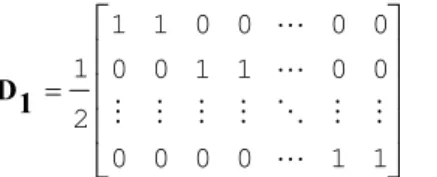
is of size M2_×N2 _{which can be}

written as [19-22]:

D = D1 D1 (2) where represents the Kronecker product, and the N/2 × N matrix _D1 represents the one dimensional (1-D) low pass filtering and down sampling . For M=N/2, we have:

(3)

From the above model, it is clear that the process of obtaining an HR image from an LR image is an inverse problem, which requires inverting the operator

_D

. It is clear that, the matrix

_D

is not a square matrix, so its direct inversion is not possible.

The target of the image interpolation process is the estimation of the vector

_f

given the vector g. According to the modern sampling theory, this process requires a correction pre-filtering step in the reconstruction process [18]. This correction filter is obtained as the inverse of the cross correlation sequence between the acquisition model filter and the reconstruction filter [18]. Unfortunately, the estimation of this correction filter in our case is difficult or even impossible. This is because our problem represented by equation (1) is an ill-posed inverse problem [19-22]. The treatment of ill-ill-posed inverse problem in the presence of noise is performed using different techniques such as regularization techniques and Wiener filtering techniques [18]. In this paper, we present an efficient regularized solution to the problem of image interpolation.

3. P

OLYNOMIAL

B

ASED

I

MAGE

I

NTERPOLATION The process of image interpolation aims at estimating intermediate pixels between the known pixel values as shown in Figure 2. To estimate the intermediate pixel at position x , the neighboring pixels and the distance s are incorporated into the estimation process.

For equally spaced 1-D sampled data, , many interpolation techniques can be used. The value to be interpolated, , can, in general, be written in the form [1-12]:

(4)

where is the corresponding interpolated function, is the interpolation kernel , and x and x_k represent continuous and discrete spatial distance, respectively. The values of c_k represent the interpolation coefficients, which need to be estimated prior to the interpolation process.

From the classical Sampling theory, if f(x) is band limited to (- , ) , then [4,6]:

(5)

This is known as the ideal interpolation. From the numerical computations point of view, the ideal interpolation formula is not practical due to the slow rate of decay of the interpolation kernel sinc(x). So, approximations such as the bicubic and cubic spline interpolation techniques are used as alternatives [1-13].

As shown in Figure 2, we define the distance between x, x_k and x_k+1 as [6,13,22]:

(6)

For the Bicubic and Cubic spline image interpolation algorithms we have [6,13,22]:

i- Bicubic

(7)

ii- Cubic Spline

(8)

For the case of bicubic interpolation, the sample values are used as the interpolation coefficients. On the other hand, cubic spline interpolation requires the estimation of the interpolation coefficients using a digital filtering step prior to the interpolation process [1-13]. In image interpolation, these techniques are performed row-by-row then column-by-column.

4. R

EGULARIZED

I

MAGE

I

NTERPOLATION

In section II, we have concluded that the image interpolation problem for CCD captured images is an inverse problem. An inverse problem is characterized as ill- posed when there is no guarantee for the existence, uniqueness and stability of the solution based on direct inversion. The solution of the inverse problem is not guaranteed to be stable if a small perturbation of the data can produce a large effect in the solution. Image interpolation belongs to a general class of problems that were rigorously classified as ill-posed problems. Regularization theory, which was basically introduced by Tikhonov and Miller, provides a formal basis for the development of regularized solutions for ill-posed problems [23,24]. The stabilizing function approach is one of the basic methodologies for the development of regularized solutions. According to this approach, an ill-posed problem can be formulated as the constrained minimization of a certain function, called stabilizing function [23,24]. The specific constraints imposed by the stabilizing function approach on the solution depend on the form and the properties of the stabilizing function used. From the nature of the problem, these constraints are necessarily related to the a priori information regarding the expected regularized solution.

According to the regularization approach, the solution of equation (1) is obtained by the minimization of the cost function [24]:

(9)

where

_C

is the regularization operator and is the regularization parameter .

This minimization is accomplished by taking the derivative of the cost function yielding:

(10)

The superscript ‘t’ refers to matrix transpose.

Solving equation (10) for that that provides the minimum of the cost function yields:

(11)

where (12)

The rule of the regularization operator

_C

is to move the small eigenvalues of

_D

away from zero while leaving the large eigenvalues unchanged. It also incorporates prior knowledge about the required degree of smoothness of f into the interpolation process.

The generality of the linear operator

_C

allows the development of a variety of constraints that can be incorporated into the interpolation operation. For instance:

a: C=I. In this case the regularized solution reduces to the regularized inverse filter solution, which is named the pseudo inverse filter solution, and it is represented as [24]:

(13)

b: C = [finite difference matrix]. In this case, the operator

C is chosen to minimize the second order (or higher order)

difference energy of the estimated image [24]. The 2-D Laplacian illustrated in Figure 3 is preferred for minimizing the second order difference energy. The 2-D Laplacian is the most popular regularization operator. It is the used operator in the paper

Figure 3: The 2-D Laplacian operator.

c- C =[eye model]. If the interpolated image is required to be appealing to the human eye from a perceptual viewpoint, the operator C is chosen as a block circulant matrix whose properties in the Fourier domain match the spatial frequency response of the human visual system [24]. The regularization parameter controls the trade-off between fidelity to the data and the smoothness of the solution.

One of the possible previously suggested solutions to this problem is to use a successive approximation for the solution, which can be implemented using the following equation [20]:

(14)

where f_i is the obtained HR image at iteration i and is a convergence parameter. This method is a good solution that avoids the large computational complexity involved in the matrix inversion process in equation (11). The drawback of this method is the computational time where a large number of iterations is required to get a good HR image.

In this paper, we suggest another solution to the regularized image interpolation problem. This solution is implemented by the segmentation of the LR image into overlapping segments and the interpolation of each segment separately using equation (11) as an inversion process. It is clear that, if a global regularization parameter is used a single matrix inversion process for a matrix of moderate dimensions is required because the term is independent on the image to be interpolated. Thus the suggested solution is efficient from the point of view of computational cost.

5. E

XPERIMENTAL

R

ESULTS

In this section, several experiments have been carried out to test the performance of the suggested inverse regularized interpolation algorithm and compare it with traditional interpolation algorithms. The images used in these experiments are first down sampled and then contaminated by additive white gaussian noise to simulate the LR image degradation model given by equation (1). The LR images are then interpolated to their original size and the MSE is estimated between the obtained image and the original image. We use two measures for performance evaluation of every image interpolation algorithm implemented. These measures are the MSE and the correlation coefficient a_e for edge pixels between the original image and the interpolated image. In applying the correlation coefficient measure, a Sobel edge detection operator is applied to both the original and the interpolated images to extract edge pixels. The correlation coefficient is estimated between edge pixels in both images. The higher the correlation coefficient, the larger the ability of the image interpolation algorithm to preserve edges through the interpolation process.

Figure 4: Lenna Image: (a) Original Image (128 × 128). (b) LR image. (64 × 64). SNR=25 dB.

original and the LR images are illustrated in Figure 4. The LR image is then interpolated using bicubic, cubic spline, iterative regularized and inverse regularized interpolation techniques. The results of this experiment are given in Figure 5.

Figure 5: Interpolation Results of Lenna Image: (a) Bicubic. MSE=339, ae=0.56. CPU=0.7 s.

(b) Cubic Spline. MSE= 342, ae=0.57. CPU=1.1 s.

(c) Iterative Regularized (100 iterations). MSE= 313, a_e=0.66. CPU=8.6 s.

(d) Inverse Regularized. MSE=223, a_e=0.78. CPU= 17.2 s.

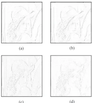
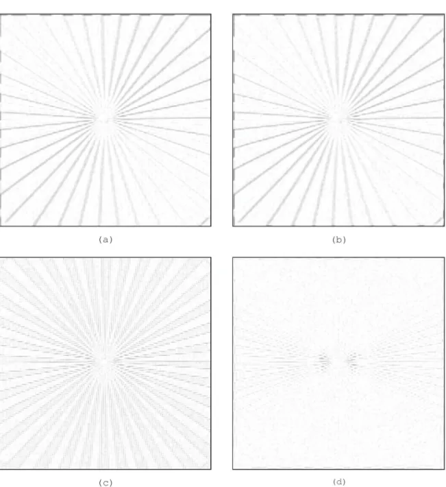
Figure 6: Error Patterns For Lenna Image Interpolation. (a) Bicubic. (b) Cubic Spline. (c) Iterative Regularized.

(d) Inverse Regularized

An error image is also estimated between the original image and each of the interpolated images. If the interpolation is ideal, all the pixel values of this error image must be zero. In this experiment, the error images are inverted and displayed in Figure 6. These error images reveal the ability of the suggested inverse regularized interpolation algorithm to preserve edges. It is clear from these results that the suggested algorithm gives better results than traditional techniques. The values of the MSE, the edge pixels correlation coefficient and the computation time using a 1 GHz processor are included with the figures for each interpolation technique. Several other experiments have been carried and the results are given in Figures 7 to 15.

Figure 7: Building Image: (a) Original Image (128×128) (b) LR image. (64×64). SNR=25 dB.

Figure 8: Interpolation Results of Building Image (a) Bicubic. MSE=1234, ae=0.22. CPU=0.7 s

(b) Cubic Spline. MSE=1304 , a_e=0.39. CPU=1.1 s (c) Iterative Regularized (100 iterations). MSE=878 , ae=0.5.

CPU=8.6 s

Figure 9: Error Patterns For Building Image Interpolation. (a) Bicubic. (b) Cubic Spline. (c) Iterative Regularized.

(d) Inverse Regularized.

In our experiments, the inverse regularized image interpolation approach is tested on the available LR images with a global regularization parameter =0.001. The LR image is segmented into overlapping blocks of size 12×12 pixels each. Each block is interpolated separately to the size of 24× 24 pixels and 8 pixels are removed from the four sides of each block to yield a small block of size 8×8 in order to avoid the edge effects. By the process of segmentation and the usage of a global regularization parameter, this technique requires a single matrix inversion of size 576×576 which is a moderate size. We have found that the size of 12×12 is the best choice. If we choose blocks of smaller dimensions, we will not be able to remove edge pixels to avoid edge effects. If we use blocks of larger dimensions the matrix required to be inverted will be of dimensions larger than 576×576 which will be difficult and time consuming. The size of the matrix to be inverted is fixed regardless of the size of the LR image. For the case of iterative regularized image interpolation, we use a regularization parameter =0.001 and a convergence parameter =0.125.

For interpolating an image of size 64×64 to size 128×128, the matrix will be of dimensions 4096×4096. If the LR image is of dimensions 128×128, the same matrix will be of dimensions 16384×16384. It is clear that the computational cost for iterative regularized image interpolation increases largely if the LR image dimensions increase, while that for inverse regularized interpolation approach will remain linearly proportional to the LR image dimensions.

The effect of the choice of the global regularization parameter in both iterative and inverse regularized image interpolation approaches is studied for the different used

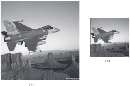
Figure 10: Plane Image: (a) Original Image (256×256). (b) LR image. (128×128). SNR=25 dB.

images and the results are given in Figures 16 and 17. It is clear that the effect of on MSE is small for in the range of 10-5 _{to 10}-2 _{for the iterative solution and in the range of}

10-5 _{to 1 for the inverse solution. The performance of the}

as the Lanczos and the Mitchell algorithms. Results of these experiments are tabulated in tables (1) and (2). These results reveal the superiority of the suggested inverse regularized image interpolation approach to the commercially available techniques.

6. C

ONCLUSION

This paper suggests an efficient implementation of the regularized image interpolation problem as an inverse problem. The suggested implementation reduces the computational cost of the image interpolation problem to a single matrix inversion problem of moderate dimensions. The obtained results using the suggested regularized image interpolation algorithm is compared to the results using the iterative regularized image interpolation algorithm and the traditional polynomial based image interpolation algorithms. The suggested implementation of regularized image interpolation has proved to be superior to polynomial based image interpolation techniques from the MSE point of view and from the visual quality point of view. It has also proved to be superior to the iterative regularized image

interpolation from the computational time point of view when the dimensions of the image to be interpolated are large. The suggested implementation has higher edge preservation ability than other interpolation algorithms.

R

EFERENCES

[1] M. Unser, A. Aldroubi, and M. Eden. B-Spline Signal Processing: Part I- Theory. IEEE Trans. Signal Processing. 41(2): 821-833, Feb. 1993.

[2] M. Unser, A. Aldroubi, and M. Eden. B-Spline Signal Processing: Part II-Efficient Design and Applications. IEEE Trans. Signal Processing. 41(2): 834-848, Feb. 1993.

[3] M. Unser. Splines A Perfect Fit For Signal and Image Processing. IEEE Signal Processing Magazine, Nov. 1999.

[4] P. Thevenaz, T. Blu and M. Unser. Interpolation Revisited. IEEE Trans. Medical Imaging. 19(7): 739-758, July 2000.

Figure 11: Interpolation Results of Plane Image. (a) Bicubic. MSE=141, ae=0.79. CPU= 2.6 s

[5] W. K. Carey, D. B. Chuang and S. S. Hemami. Regularity Preserving Image Interpolation. IEEE Trans. Image Processing. 8(9): 1293-1297, Sept. 1999.

[6] J.K. Han and H. M. Kim. Modified Cubic Convolution Scaler With Minimum Loss of Information. Optical Engineering. 40(4): 540-546 , April 2001.

[7] H. S. Hou and H. C. Andrews. Cubic Spline For Image

Interpolation and Digital Filtering. IEEE Trans. Accoustics , Speech and Signal Processing. vol. ASSP-26 , No.9, pp. 508-517, Dec. 1978.

[8] T. M. Lehman, C. Conner and K. Spitzer. Addendum: B - S p l i n e I n t e r p o l a t i o n i n M e d i c a l I m a g e Processing. IEEE Trans. Medical Imaging. 20(7): 660-665 , July 2001.

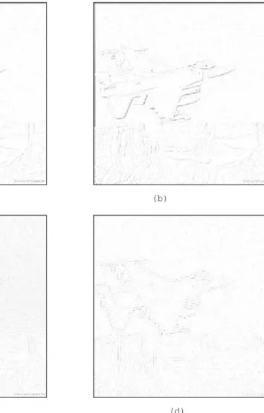
Figure 12: Error Patterns For Plane Image Interpolation.

(a) Bicubic. (b) Cubic Spline. (c) Iterative Regularized. (d) Inverse Regularized.

[9] B. Vrcelj and P.P. Vaidyanathan. Efficient Implementation of All-Digital Interpolation. IEEE Trans. Image Processing. 10(11): 1639-1646, Nov. 2001.

[10] T. Blu, P. Thevenaz and M. Unser. MOMS:Maximal-Order Interpolation of Minimal Support. IEEE Trans. Image Processing. 10(7):1069-1080, July 2001 .

[11] E. Meijering and M. Unser. A note on Cubic Convolution Interpolation. IEEE Trans. Image Processing. 12(4):477-479, April 2003.

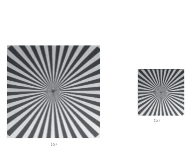
Figure 13: Test Pattern Image. (a) Original Image (128×128). (b) LR image. (64×64). SNR=25 dB.

[13] G. Ramponi. Warped Distance For Space Variant Linear Image Interpolation. IEEE Trans. Image Processing. vol.8, pp. 629- 639, 1999.

[14] S. E. El-Khamy , M. M. Hadhoud, M. I. Dessouky, and F. E. Abd El-Samie. Adaptive Image Interpolation Based on Local Activity Levels. the 20th _National

Radio Science Conference, (NRSC’2003), Cairo, March 18-20, 2003.

[15] S. E. El-Khamy , M. M. Hadhoud, M. I. Dessouky, B. M. Salam, and F. E. Abd El-Samie. A New Edge Preserving Pixel-by-Pixel (PBP) Cubic Image Interpolation Approach. 21th _{National Radio Science}

Conference, (NRSC’2004), Cairo, March 16-18, 2004. [16] S. E. El-Khamy , M. M. Hadhoud, M. I. Dessouky, B. M. Salam, and F. E. Abd El-Samie, “ A New Approach For Adaptive Polynomial Based Image Interpolation” Accepted for publication in the International Journal of Information Acquisition. [17] S. E. El-Khamy , M. M. Hadhoud, M. I. Dessouky,

B. M. Salam, and F. E. Abd El-Samie. An Adaptive Cubic Convolution Image Interpolation Approach.

Submitted for publication, Journal of Machine Graphics and Vision, July 2005.

[18] M. Unser , A. Aldroubi. A General Sampling Theory for Nonideal Acquisition Devices. IEEE Trans. Signal Processing. 42(11):2915-2925, Nov. 1994.

[19] W. Y. V Leung, P. J. Bones. Statistical Interpolation of Sampled Images. Optical Engineering. 40(4):547-553, April 2001.

[20] J. H. Shin, J. H. Jung, J. K. Paik. Regularized Iterative Image Interpolation And Its Application To Spatially Scalable Coding. IEEE Trans. Consumer Electronics. 44(3): 1042-1047, August 1998.

[21] S. E. El-Khamy , M. M. Hadhoud, M. I. Dessouky, B. M. Salam, and F. E. Abd El-Samie. Optimization of Image Interpolation as an Inverse Problem Using The LMMSE Algorithm. Proc. of IEEE MELECON’2004, Dubrovnik, Croatia, May 12-15, pp. 247-250, 2004. [24] H.C. Andrews and B.R. Hunt, Digital Image

Restoration. Englewood Cliffs, NJ: Prentice- Hall, 1977. [25] 2005 ACD Systems, ACD, http://www.

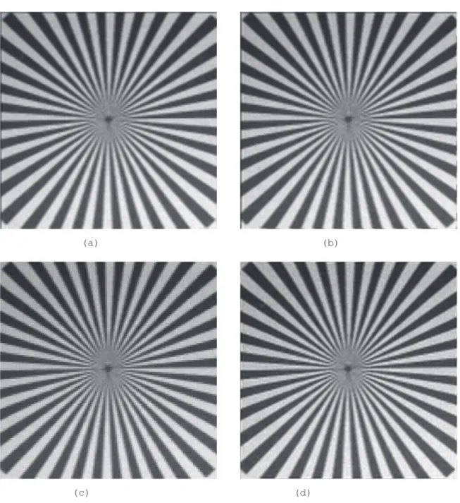
Figure 14: Interpolation Results of Test Pattern Image. (a) Bicubic. MSE=315, ae=0.47. CPU=2.6 s.

Figure 16: Effect of regularization parameter on iterative regularized image interpolation

Figure 18: MSE vs. SNR for the Lenna Image.

Figure 20: MSE vs. SNR for the Plane Image.

Table 1: Interpolation results for different noise free images.