robustness of a scale-free network when links are irreversibly removed after failing. Due to inherent charac-teristics of the fuse network model, the sequence of links removal is deterministic and conditioned to fuse tolerance and connectivity of its ends. It is a different situation from classical robustness analysis of complex networks, when they are usually tested under random fails and deliberate attacks of nodes. The use of this system to study the fracture of elastic material brought some interesting results.
DOI:10.1103/PhysRevE.72.046709 PACS number共s兲: 05.10.⫺a, 89.75.⫺k, 02.70.⫺c
I. INTRODUCTION
Material science and engineering have always been con-cerned with robustness and durability of materials where a trade off involving energy consumption, costs, and mechani-cal reliability is to be optimized. The damage and fracture of materials always involve economic and human costs. Crack-ing of glass, corrosion of metallic structures and tools, the aging of concrete, and the failure of fiber networks are just a few of many everyday stressing situations leading to material failure.
Different classes of materials have different mechanical and thermal properties. Ceramics are incredibly rigid and thermally resistant, but their failure is catastrophic for their lack of plasticity. Metals are much softer than ceramics, but have thermal restrictions and are way too heavy for certain uses. Weight is not usually a problem with polymers, but excessive creep under heat and degradation under ultraviolet radiation often limit their usage. In that scenario, composites may arise as a solution, combining the best of two materials. The idea is not new. Wood itself is a fibrous composite: cellulose fibers in a lignin matrix. The cellulose fibers have high tensile strength but are very flexible共i.e., low stiffness兲, while the lignin join the fibers and furnishes the stiffness. Rocks, concrete, Portland cement are all successful examples of composite materials关1兴.
So it seems to be a fact that inhomogeneity in materials is in many cases desirable. That leads to the problems concern-ing structures characterized by the lack of conventional geo-metrical order. Actually, several statistical models for the fracture of disordered media have been proposed and ex-plored in the last few decades共see 关2兴 for a good review兲. One of them is the random fuse network 关3–8兴, described below, that makes use of the similarity between Hook’s law and Ohm’s law, trying to apprehend the role of heterogeneity at a mesoscopic level taking to macroscopic failure in elastic materials. The network itself is regular, usually square, the disorder is introduced via dilution 共a certain fraction of the fuses is removed兲and/or attributing different characteristics
to each fuse. In the present work, the disorder is introduced by using a irregular geometry for the network. Not a random network, but a scale free network共SFN兲.
SFN’s have been found to lie behind the structure of many natural and artificially created networks 关9兴: www 关10,11兴, internet routers关12兴, proteins关13兴, and scientific collabora-tions关14兴, just to name a few. The main features that distin-guish these complex networks from “ordinary” ones are their small-world character 关15兴 and the scale-free degree distri-bution关16兴.
The original model to create SFN’s was proposed by Al-bert and Barabasi关17兴and was based on growth and prefer-ential attachment. At each time step a new node is added to the network and attaches itself tom already existing nodes with probability proportional to their incidence degrees. With this simple recipe, a scale-free network with degree distribu-tion of exponent 3 is obtained. Some changes and new mod-els have also been proposed, allowing a control of the char-acteristic exponent and catching different dynamics for growth and even competition between the nodes of the network关18兴.
Given the abundant examples of complex networks in na-ture, the problem of attacks on complex networks has at-tracted a lot of attention recently 关19–22兴. It has been ob-served that scale-free networks display an exceptional robustness against random node failure, but show poor per-formance against preferential node removal 共the most con-nected nodes are preferentially removed兲.
The robustness of SFN’s has also been evaluated using the fiber bundle model关2兴as a scenario 关23,24兴. The nodes were fibers that broke when the load imposed was greater than their individual threshold. But, again, the nodes共fibers兲 were the entities to be removed. As in the case of the reli-ability evaluation of power transmission systems 关25–27兴, the present work strives to evaluate the robustness of net-works when the links, and not the nodes, are subjected to overload. Power systems, however, are not scale-free net-works. And, as far as the authors know, this is the first time scale-free networks have their robustness tested under deter-ministic link failure. If the system is also thought to mimic a fiber reinforced material, it makes a lot more sense thinking of fibers as links instead of nodes, for it is hard to imagine that a single fiber could locally share its load with as many fibers as a hub in a SFN.
*Electronic address: [email protected]
†
II. MODEL
In the classical random fuse network model, fuses are placed at random on the bonds of ad-dimensional hypercu-bic lattice. Figure 1 shows the two-dimensional case. Two busbars are placed across the top and the bottom rows of the network and a voltage difference V is applied between the two bars. The external voltage made sufficiently large will burn a fuse or a few of them and eventually take the system to a complete rupture or breakdown, when no current flows. The fuses may be identical, i.e. have identical conductiv-itygjand identical toleranceicj, in which case the disorder is introduced by diluting the links in the network, respecting the percolation limit, as in Fig. 1共a兲.
A different array may be set with a regular square net-work, as in Fig. 1共b兲. In that case, disorder comes with a statistical distribution of fuse characteristics 共conductivity and/or tolerance兲.
In the present work, the disorder element is simply the network topology, for SFN’s are marked by a power-law de-gree distribution and short characteristic length 关9,28,29兴. The possibilities concerning the connectivities of both termi-nals of each fuse are unlimited共actually it is limited by the maximum connectivity, which, by its turn, is only limited by the size of the network兲.
The fuse network in square lattices clearly establishes two sets of nodes that are connected to the source terminals via two bus bars, usually the top and the bottom rows of nodes. For a complex network, however, this matter is not clear. What is proposed here is starting from an intuitive notion of peripheral and central regions in the network; we will study three different cases of loading.
The peripheral region is now declared to be the set of all nodes with connectivityk=m. These are the nodes that were
never connected after being added to the network. They cor-respond to the nodes with the lowest connectivity in the net-work and, most likely, the last nodes added to it.
On the opposite hand, the the central node is defined as the most connected one.
Based on these definitions, three different loading cases are studied:
共1兲 One terminal of the voltage source is connected to the central node and the other terminal, to the peripheral nodes. 共2兲 The peripheral region is divided into two sets with the same number of nodes共or differing by one兲 and each set is connected to a terminal of the voltage source.
共3兲 A few randomly chosen nonperipheral nodes are con-nected to one terminal of the voltage source and the periph-eral region is connected to the other terminal.
The peripheral nodes are actually merged into a single node, in cases共1兲 and共3兲, or two nodes, in case 共2兲. These are sometimes referred as the periphery terminal or the pe-riphery along the text.
III. METHODS
To deal with the terrifying problem of analyzing the com-plex circuit created by a scale-free network it was made broad use of graph theory. The analogy between an electric circuit and a directed graph with across and through vari-ables is complete关30兴. Kirchhoff’s current and voltage laws are general postulates regarding incidence and circuit prop-erties of directed graphs.
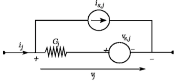
The fuse network circuit can be mapped onto a directed graph, where each link corresponds to a circuit element 共a resistor or a voltage source兲and the nodes simply correspond to circuit nodes. Each link is attributed a conductivity value Gj and has two variables: the current 共through兲 ij and the voltage共across兲 vj. Kirchhoff’s current law is simply stated
as
Ai=0 共1兲
where A is the reduced incidence matrix of the oriented
graph representing the network.
A typical element of a resistive network关30兴is shown in Fig. 2.
The subscript j indicates the jth element of the network and the subscript s indicates a generator or source. From Fig. 2, it follows
ij=Gjvj+is,j−Gjvs,j, j= 1,2, . . . ,e. 共2兲 ebeing the number of elements in the circuit or arcs in the graph. The set of equations共2兲may be written in the vector form
i=Gv+is−Gvs, 共3兲
where the conductivity matrixG is a diagonal matrix with each elementGj jcorresponding to the conductivity of the jth circuit element.
The node analysis of the network, corresponding to Kirchhoff’s current law Eq.共1兲, can now be expressed by
AGv+Ais−AGvs=0. 共4兲
Now, ifvndenotes the nodes voltages relative to a chosen datum node, the vector v of voltages across each element may be written as
v=Atvn. 共5兲
Using共5兲in共4兲and considering that our circuit is only fed by a voltage source共is=0兲, it comes
AGAtv
n=AGvs. 共6兲
Defining the node admittance matrixY=AGAt, the net-work node analysis results in the expression
Yvn=in 共7兲
wherein=AGvs.
Since Y is invertible, vn can be found by means of Eq. 共7兲. Equation 共5兲 will then give v and Eq. 共3兲 will finally
providei, the vector of currents through each element.
Once created the scale-free network, each one of its e links is made a fuse, all having the same conductivity Gj = 1 and the same tolerance ic,j= 1. An external voltage vs
= 1 is then applied to this network, adding an extra element to the network. The vectorvs, corresponding to the voltage
sources, has only one nonzero element, that is its 共e+ 1兲th
entry. In order to have Y invertible, the external voltage source has to be nonideal and its conductivity is also made unitary.
The test procedure for a single network begins with the inversion ofYto obtainvn,vand finallyi, by means of Eqs.
共7兲,共5兲, and共3兲. The external voltage vsis always set to 1,
but the real voltage at the terminals of the voltage source is
ve+1=vs−Ge+1ie+1=vs−ie+1共recalling that the indexe+ 1
de-notes the extra element added, that is, the voltage source兲. The hottest fuse is the one with the maximum ratio =ij/ic,j, from now on, called max. So, the external 共real兲 voltage to burn the hottest fuse isV=ve
+1/max, and the total current I=ie+1/max. The burning of a fuse means it is irre-versibly removed from the network. The currents are recal-culated and again the hottest fuse is removed for a new value of V and I, which will define a sequence 共Vm,Im兲, with m ranging from 1 to the last burning of a fuse, corresponding to the network breaking apart and no more current being con-duced through it.
After themth fuse connecting node rto node s is burnt and removed from the network, the new admittance matrixY
will be given by
Ym+1=Ym−Grswwt
wherewis a vector whose elements are given by FIG. 3. Typical picture at final failure of network in loading case
1. Heavy lines are the burnt fuses. The central node is at the top marked by a large arrow departing from it. The periphery terminal is on the right, marked by a large arrow. The network is made small only for visualization purposes.
wr= 1
ws= − 1
wj= 0, for j⫽randj⫽s.
andGrsis the conductance of the fuse that connects noderto nodes. Significant computational advantages can be gained if the inverse of Ym is simply updated by the well-known Shermon-Morrison-Woodbury formula.关31,32兴
Ym
+1 −1
=Ym−1+
冉
frs uut
共1 −Grswtu兲
冊
whereu=Ym−1w.
The whole process is carried out using Scilab, the scien-tific software package, which has built-in graph tools.
IV. RESULTS AND DISCUSSION
A. Load mode 1
Load mode 1, as described earlier, refers to a central con-fluence of load, meaning that the links incident to this central load are the most likely to be overloaded. Figure 3 confirms that. It shows a small network at the end of simulation, when no more current is flowing because the system has broken down.
This is the typical result; all links incident to the central node failed. Sometimes an extra link would break, as in this case共the one at the very bottom兲.
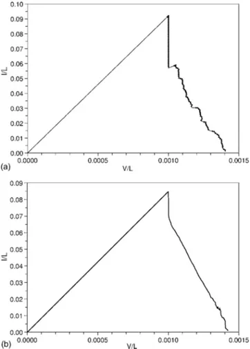
The plot of current vs voltage for this load mode is shown in Fig. 4.L, inI/LandV/L, is the number of nodes, set to 1000 in all simulations in this section.
The profile seen in Fig. 4共b兲 resembles the stress-strain curve of a elastic material reinforced with fibers made of a tougher elastic material共like carbon fiber reinforced glass关2兴 and carbon fiber in carbonaceous matrix关1兴兲—the fibers pre-venting the catastrophic one-crack failure.
B. Load mode 2
This mode, described earlier, would suggest escaping the total confluence toward the central node as seen in case 1. Nevertheless the rupture will be defined in one of the periph-eral neighborhoods, as can be seen in Fig. 5.
Any imbalance between the two peripheral halves will trigger an avalanche in one of the “sides.”
Figure 6 shows the behavior of theIvsVcurve during the FIG. 5. Typical picture at final failure of network in loading case
2. Heavy lines are the burnt fuses.Cindicates the central node;P1 andP2 are the two halves of the peripheral region. The network is made small for easier visualization.
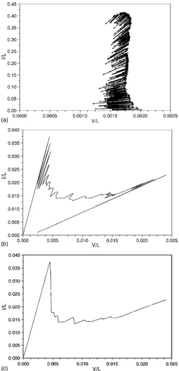
burning sequence for this case. In Fig. 6共a兲 it is possible to see significant oscillations observed for a single network. The arrows explicit the burning sequence. When averaged over 100 samples, the oscillations are significantly smoothed, as shown in Fig. 6共b兲.
If a voltage controlled test is considered, whereVis made to increase monotonically and never decrease, the curve ob-tained is the one shown in Fig. 6共c兲. The mechanical corre-spondent would be the strain controlled test. It shows, in this case, a smooth transition not observed in either two other load cases. Mechanically it would represent fiber bridging, after matrix extensive microcracking, followed by fiber bundle failure关1,33兴.
C. Load mode 3
Another situation is described by case 3, also described earlier. Here the confluence toward the central node is re-lieved by setting a small fraction共⬃1 %兲of nodes to divide the flow toward the ”central” terminal -as the one opposed to the periphery. The result is a spread of burned fuses as can be seen in Fig. 7.
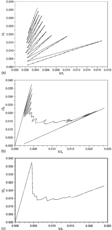
The plot of current versus voltage in this case shows an interesting oscillation as can be seen in Fig. 8共a兲 and 8共b兲. For a single sample, it is interesting to note that after the first burn of a fuse, the three next fuses will burn in a decreasing sequence of overall tolerance 共lower currents兲 of the net-work. Next, a significant raise in tolerance is seen, to be followed again by a decreasing sequence.
Along each lowering tolerance sequence, the overall con-ductivity of the network seems to remain nearly unchanged, since the values ofIandV, in the sequence, lie on a straight line that intercepts theVaxis next to the origin.
Averaging over 100 samples, I vs V curve still displays strong oscillations关Fig. 8共b兲兴. When the voltage controlled test is considered, with monotonically increasing V, the curve obtained is the one shown in Fig. 8共c兲.
V. CONCLUSIONS
The inherent inhomogeneity of scale-free networks has shown interesting consequences to the robustness of systems
described by this kind of networks when their links are under load and subject to deterministic failure. Their characteristic distribution of incidence degrees has proved to be a major disorder element, with no need of further inhomogeneity dis-tributions such as different load thresholds or different load response for the links.
Three different load modes have given place to three dis-tinct breaking profiles. The disdis-tinctions were clear in both the load concentration geometry and overall load responses. FIG. 7. Typical picture at final failure of network in loading case
3. Heavy lines are the burnt fuses.Cindicates the central node共the most connected one兲.Pdenotes the periphery andRis the terminal connected to the randomly chosen nodes. The network is made small for easier visualization.
关1兴K. K. Chawla,Composite Materials—Science and Engineering 共Springer-Verlag, New York, 1987兲.
关2兴H. J. Herrmann and S. Roux,Statistical Models for the Frac-ture of Disordered Media 共Elsevier Science Publishers, New York, 1990兲.
关3兴P. M. Duxbury, P. D. Beale, and P. L. Leath, Phys. Rev. Lett.
57, 1052共1986兲.
关4兴B. Kahng, G. G. Batrouni, S. Redner, L. de Arcangelis, and H. J. Herrmann, Phys. Rev. B 37, 7625共1988兲.
关5兴L. de Arcangelis and H. J. Herrmann, Phys. Rev. B 39, 2678 共1989兲.
关6兴G. G. Batrouni and A. Hansen, Phys. Rev. Lett. 80, 325
共1998兲.
关7兴S. Zapperi, P. Ray, H. E. Stanley, and A. Vespignani, Phys. Rev. E 59, 5049共1999兲.
关8兴S. Zapperi, H. J. Herrmann, and S. Roux, Eur. Phys. J. B 17, 131共2000兲.
关9兴R. Albert and A.-L. Barabási, Rev. Mod. Phys. 74, 47共2002兲.
关10兴B. A. Huberman and L. A. Adamic, Nature共London兲 401, 131 共1999兲.
关11兴R. Albert, H. Jeong, and A.-L. Barabási, Nature共London兲 401,
130共1999兲.
关12兴G. Caldarelli, R. Marchetti, and L. Pietronero, Europhys. Lett.
52, 386共2000兲.
关13兴H. Jeong, S. Mason, A.-L. Barabási, and Z. N. Oltvai, Nature 共London兲 411, 41共2001兲.
关14兴M. E. J. Newman, Phys. Rev. E 64, 016132共2001兲.
关15兴D. J. Watts and S. H. Strogatz, Nature 共London兲 393, 440
共1998兲.
关16兴A.-L. Barabási and R. Albert, Science 286, 509共1999兲. 关17兴A.-L. Barabási, R. Albert, and H. Jeong, Physica A 272, 173
共1999兲.
关18兴H. Stefancic and V. Zlatic, e-print cond-mat/0409648共2004兲.
关19兴R. Albert, H. Jeong, and A.-L. Barabsi, Nature共London兲 406,
378共2000兲.
关20兴R. Cohen, K. Erez, D. ben-Avraham, and S. Havlin, Phys. Rev. Lett. 85, 4626共2000兲.
关21兴A. E. Motter, Phys. Rev. Lett. 93, 098701共2004兲.
关22兴J.-L. Guillame, M. Latapy, and C. Magnien, Comparison of Failures and Attacks on Random and Scale-Free Networks 共Springer-Verlag, Grenoble, 2005兲. Lect. Notes Comput. Sci.
3544, 186–196共2005兲
关23兴Y. Moreno, J. B. Gomez, and A. F. Pacheco, Europhys. Lett.
58, 630共2002兲.
关24兴D. H. Kim, B. J. Kim, and H. Jeong, Phys. Rev. Lett. 94,
025501共2005兲.
关25兴J. Chen, J. S. Thorp, and I. Dobson, Int. J. Electron. 27, 318 共2005兲.
关26兴B. A. Carreras, V. E. Lynch, I. Dobson, and D. E. Newman, Chaos 12, 985994共2002兲.
关27兴I. Dobson, J. Chen, J. S. Thorp, B. A. Carreras, and D. E. Newman, in Proceedings of the 35th Hawaii International Conference on System Sciences, Hawaii, 2002, 共IEEE Com-puter Soc., Big Island,共2002兲.
关28兴A.-L. Barbási and E. Bonabeau, Sci. Am. 288, 50共2003兲.
关29兴A.-L. Barabsi,Linked: The New Science of Networks共Perseus Publishing, Cambridge, 2002兲.
关30兴D. E. Johnson and J. R. Johnson,Graph Theory with
Engineer-ing Applications 共The Ronald Press Company, New York,
1972兲.
关31兴G. H. Golub and C. F. van Loan,Matrix Computations3rd ed. 共The Johns Hopkins University Press, Baltimore, 1996兲. 关32兴P. Kumar, V. V. Nukala, and S. Simunovic, J. Phys. A 36,
11403共2003兲.