Figure 1 – Main outcome of this Work Project

(1)

A Work Project, presented as part of the requirements for the Award of a Masters Degree in

Management from the Nova School of Business and Economics

How can clusters help in the product type choice? The case of a specialized retail store

António Manuel Domingues Ribeiro

#1414

A project carried out with the supervision of:

Professor José António Pinheiro

(2)

1. Abstract

This work project (WP) is a study about a clustering strategy for Sport Zone. The general

cluster study’s objective is to create groups such that within each group the individuals are

similar to each other, but should be different among groups. The clusters creation is a mix

of common sense, trial and error and some statistical supporting techniques.

Our particular objective is to support category managers to better define the product type to be displayed in the stores’ shelves by doing store clusters. This research was carried out

for Sport Zone, and comprises an objective definition, a literature review, the clustering

activity itself, some factor analysis and a discriminant analysis to better frame our work.

Together with this quantitative part, a survey addressed to category managers to better

understand their key drivers, for choosing the type of product of each store, was carried out.

Based in a non-random sample of 65 stores with data referring to 2013, the final result was

the choice of 6 store clusters (Figure 1) which were individually characterized as the main

outcome of this work:

In what relates to our selected variables, all were important for the distinction between

clusters, which proves the adequacy of their choice. The interpretation of the results gives

category managers a tool to understand which products best fit the clustered stores.

Furthermore, as a side finding thanks to the clusterization, a STP (Segmentation, Targeting

and Positioning) was initiated, being this WP the first steps of a continuous process.

(4)

2

2.Introduction

Sport Zone started its commercial activity in 1977 with the opening of its first store in Gaia.

Nowadays, including outlets and franchising, it has 75 stores in Portugal (most of them

located in Algarve, Lisbon and Porto metropolitan areas). Despite also having stores with

their insignia in Spain, this analysis only targets the Portuguese market, and within this

market, we excluded both outlets and franchsings, resulting in 65 stores eligible for this

analysis.

In spite of Portugal’s small dimensions, regions across the country are very different in

terms of demographic characteristics, inter alia. This diversity indicates that it is not

adequate to have the same range of products for all the stores spread over the country, since

there are several types of clients with different needs to be satisfied. Hence, the main idea

of this WP is to group similar stores, and to smooth the product choice process of the

category managers.

As usually happens with these empirical methods, the cluster analysis was supported by a

factor analysis, to try to reduce the variable’s number, and a discriminant analysis to

reallocate some stores initially considered as outliers.

Thesis statement:

The selected variables used in the cluster analysis forcedly impact the type of products to

(5)

3

Table 1 – Variables definition

Table 2 – Variables expected impact

3. List of acronyms and initial variables definition

We reached this list of initial variables (Table 1) through the perusal of academic papers

and by attending internal meetings. A sample dataset example is presented in Appendix 1.

Our common thread was to always think on what would be the expected impact that each

variable would have in our final results, measuring this way their level of utility to the

category managers, the actual users of this WP, (Table 2).

Domains Acronym Name Description Units Type Source

C

u

st

o

me

rs B Brand Weight of the supplier brand sales per store Percentage Continuous SONAE database

P Promotions Weight of the promotion sales per store Percentage Continuous SONAE database

S Average Ticket Average expenditure per client per store EUR Continuous SONAE database

Geo g ra p h ic

T Temperature Average temperature in the district where the store is located Degree Celsius Continuous INE

C Rainfall Average rainfall in the district where the store is located MM Continuous INE

D emo g ra p h

ic I Income GDP Index of the municipality where the store is located Index number Continuous INE

G Gender Weight of the female sex in the municipality where the store is

located Percentage Continuous INE

A Age Weight of the population by intervals of age per store Percentage Discrete INE

Name Expected Impact

Brand Measures whether the cluster strategy must be to reinforce private or supplier brand.

Promotions Measures whether the cluster strategy should be to implement more promotions or less than what is happening today

Average Ticket

Stores with a high Average Ticket have an actual client with more purchasing power. This variable is heavily conditioned by the range of

products of each store (“supply”).

Temperature

Measures whether the cluster strategy should aim towards a shorter or a longer summer/winter. Moreover, depending on the temperatures,

some products might make more sense to be displayed ( e.g. in high temperatures, products like carded clothing must have less weight)

Rainfall Depending on the rain affecting each district, it might be advisable to sell certain types of product (e.g. rain clothing)

Income

Whenever a store is inside a municipality with a high GDP Index, the potential client will be one with more disposable income to spend. In

that sense, more expensive items should be displayed. Furthermore, Income in contrast to Average Ticket represent the potential client

Gender Allows defining the proportion of female and male items.

Age

Age ranges provide deeper understandings over the age ranges with more preponderance amidst the municipality where the store is located.

(6)

4

4. Literature Review

Wedel, Michel. Kamakura, Wagner, Böckenholt, 2000, state that for a company it is almost

impossible to make a customized targeting to all its range of customers. By association, we

also think that when a company has numerous stores to manage, to define an individual

store strategy, is just too costly. As said before, and looking to the specialized store income

statement, if an individualized strategy was implemented, the time and money spent would

turn out to be a financial burden too big to surpass. Crossing into this issue, doing store

clusters seemed to be perfectly suitable and less time and money consuming than to treat

each store separately.

Mendes and Cardoso, 2006, purposed dividing the variables in three groups (Location and

Outlet Attributes, Influence Area Characterization and Clients Characteristics). Instead of

having three group types, our analysis contains 4 domains: Clients; Geographic;

Demographic and Competition. Wedel, Michel. Kamakura, Wagner, Böckenholt, 2000,

also highlight that soft data is considered to be as important as hard data. In that sense, we

used in our analysis both the database given and the category manager’s experience.

Mendes, Armando. Cardoso, Margarida. 2006 also propose three methodologies to cluster

supermarkets: a priori; a posteriori and an interactive. All of them rely on manager’s

expertise but in different ways. As this study concluded, an interactive approach consisting

on having expert’s contribution in both variables decisions and evaluation of the clusters

validity/stability, performs the best possible results. Therefore, I used the knowledge of

category managers (questionnaires) for this purpose (Wedel and Kamakura, 2000; Jain and

(7)

5

2003, Henning and Christlieb, 2002 and Jones, 1996.) on “Visual cluster validation”,

support our analysis.

Despite a correct methodology, I have encountered some downsides in Mendes, Armando.

Cardoso, Margarida, 2006. In fact, they only used Pearson correlation matrix to reduce the

number of variables. To overcome this situation, factor analysis was considered in our

analysis.

In what relates to the methodology used, we opted not to use regressions trees as a valid

option because they are not the appropriate for small datasets (Bay and Pazzani, 2000). As

in the paper conducted by Lockshin, Lawrence. Spawton, Anthony. Macintosh, Gerrard,

1997, we also used the three step methodology applied by Singh (1990), to assure both

validity and stability of the clusters: 1) division of the data into two sub-samples; 2) Use

Ward method followed by K-means; 3) Identification and characterization of each cluster.

Although the first step was compromised (division of the dataset into two subsamples) due

to a short dataset, we continue using the remaining steps to obtain the final clusters

solution. Thus, with Ward method we were able to correctly identify the optimal number of

clusters (6) which was in line with category manager’s recommendations of not having too

many clusters. This then served as an input to the K-means non-hierarchical method

(Johnson & Wichern, 2002) to obtain the final cluster membership.

At last, discriminant analysis (Tabachnick & Fidel) was used to reallocate the outliers and

(8)

6

5. Preliminary analysis

When performing an explanatory data analysis (Appendix 2), we can observe that the

variables which have a bigger standard deviation are the Average Ticket, the Income and

the Competition. In case of outlier’s inexistence, these variables will in a second stage have

a bigger role in differentiating the clusters. On the other hand, the variables which have the

lowest standard deviation are “age intervals”.

Both Skewess and Kurtosis tests point out different things. While the first one verifies if the

distribution is symmetric, the second one provides information about the peakedness of the

distribution. The variables which have values clustered to the right (negative skewess

statistic) are: Average Ticket, Temperature and some of the age intervals. All the others are

clustered to the left.

Relatively to the kurtosis test, the statistics with negative values indicate that those same

values are more located in the tails and less in the center. The variables having this type of

value distribution are: Brand and Rainfall. These variables will, as explained ahead, be

standardized although their fitness to this transformation isn’t as good as the others.

(9)

7

6. Correlations matrix

To see if there are redundant variables in the 4 domains, we did a correlation matrix

(Appendix 3) through Pearson correlation coefficient. We fixed - >70%/<-70% - as the

limit from which two variables could be considered as having a high correlation. The boxes

painted in green represent a positive high correlation (> 70%). On the other way around, the

red boxes represent a high negative correlation (< -70%).

As Appendix 3 shows, Average Ticket and Brand have a correlation of 73% and

Temperature and Rainfall a correlation of -72%. Our choice of eliminating one of these two pairs could turn out to be arbitrary because statistically they perform very identically.

However, with the help of the questionnaire made to the category managers (section 8), we

were able to eliminate the ones presenting the worst scores. Therefore, Average Ticket and

Rain Fall were eliminated from our initial list of variables.

Regarding the age intervals, if we were going to eliminate variables until no correlations

were left, a lot of variables would disappear. The solution found was to condense the

information by using factor analysis on the different age group intervals as shown in the

next section.

In respect to the other variables, none of them presented correlations among themselves.

(10)

8

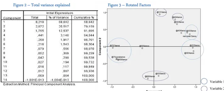
Figure 2 – Total variance explained

7. Factor Analysis

We applied a Factor Analysis to the variables age groups to reduce their number from 14

age intervals to 2 or 3 factors (new variables). This way, all the information is condensed,

simplified and it might be even possible to discover latent dimensions.

The relevant outcome of the Factor Analysis was the following:

As described in Figure 2, the two first components explain a high share of the total variance

of all the variables (79%). This was basically the rule to decide how many factors we

should retain, and so, we retained the two first factors.

In Figure 3, we observe that all the variables were gathered around the 2 retained factors

(Figure 2) which demonstrates that the factorial analysis was feasible. We also did a Table

with the coefficients of each variable in the factors (Appendix 7), to understand at what

extent the factors explained the variables. While the first factor explains:“<15”;”25

-29”;”30-34”;”35-39”;”65-69”;”70-74”;”>75”, the second explains “15-19”;”40-44”;“55

-59”;”60-64”. To allow a better comprehension of the factors we named the first factor as

being “Grandparents and their grandchildren” and the second as “Mothers and Fathers”.

(11)

9

8. Questionnaire

Despite the quantitative approaches used so far, we still had too many variables. To

conclude our choice of variables, we decided to use as an input the several years of

experience of the category managers (Mendes, Armando. Cardoso, Margarida. 2006).

Usually with cluster analysis, we start with a pool of variables and test different

combinations until reaching the results that best respond to our objectives. This makes the

variables choice simply arbitrary. In order to rest assure that the utility being given to the

category mangers would be maximized, we did this questionnaire (Appendix 4) to help

choosing the best variables.

We presented the 15 category managers with a

questionnaire. This empirical questionnaire asked

category managers to rate the variables on a scale from

1 to 4, being 1 not relevant and 4 very important. The

total scores are in Table 4 and the main conclusions

were: Gender, Rainfall and Average Temperature had

the worst scores and were eliminated from our analysis.

As seen in Appendix 3, Brand and Average Ticket were

correlated and so we picked the one with the highest

score (Brand). Also, category managers recommended

using competitor’s proximity and distance to coastline

as two important variables.

These inputs were considered in our final variables list.

Table 3 – Questionnaire results

Name Description Total

Score

Brand

Percentage of the supplier brand sales

per store

55

Promotions

Percentage of the promotion sales per

store

50

Average Ticket

Average expenditure per client per store

44

Temperature

Average temperature in the district where

the store is at

40

Rainfall

Average rainfall in the district where the

store is at

37

Gender

Percentage of the feminine sex in the municipality where

the store is at

37

Income

Income of the municipality where

the store is at

46

Age

Percentage of each age group

(12)

10

9. Final variables list

Our final variables list is then composed by the variables with the best ranking in the

questionnaire, plus the age factors and finally the recommendations of the category

managers were also attended. Keeping this last one in mind, we created two proxies’ to

represent those concepts: distance to nearest competitor and amplitude. Definition of these

two new variables (Table 4):

Table 4 – New variables definition

We can now think about what would be the impact that these variables would have in the

clusters strategy and if they are worthwhile to the analysis (Table 5):

We also checked the correlations of these two variables with all the others and no

correlations were identified. Concluding, our final variables list is as follows:

Promotions; Amplitude; Brand; Income; Age factors 1 & 2 and Competitors distance.

Domains Acronym Name Description Units Type Source

Geographic R Amplitude Temperature amplitude of the district where the store is at Degree

Celsius Continuous INE

Competition K Competitors

distance

Minimum distance of each store to a direct competitor

(Decathlon & SportsDirect) Kilometers Continuous SOMA

Table 5 – New variables expected impact

Name Impact

Amplitude

Allows understanding whether a store is near the coast or in the country’s interior. Proximity to the sea leads to milder

temperatures which impact, for example, the type of clothing and if there is a need for higher differentiation between seasons or

not (more or fewer collections).

Competitors

distance

The distance from each store to the nearest competitor is a measurement on how it should react as long as price and product range

(13)

11

10. Variables standardization

We opted to use z-scores during the cluster analysis for mostly one reason. The fact that the

measurement units differ in each variable will make some variables to bear more weight in

the analysis than others. Standardizing them is the usual solution.

11. Outlier analysis

11.1 Outliers identification

To identify the outliers, we used Z scores, one of the outlier’s selection methods, to

eliminate the stores with more than 3 or less than -3 for each of the variables. Whenever a

store’s value overtakes these boundaries, it was considered as an outlier. In table 6, outliers

for each of the variables, are represented. All these stores are going to be eliminated from

our initial information and, as shown further ahead, they will be replaced in the computed

clusters by using discriminant analysis.

Final Variables Correspondent Outliers

Factor 1 age Rio Tinto; Castelo Branco

Factor 2 age Castelo Branco

Promotions None

Income Colombo; Spacio Olivais; Vasco da Gama; Amoreiras

Competitors distance Bragança; Beja

Brand None

Temperatures range None

(14)

12

12. K-means supported by Ward method

The main difference between K-means and all the hierarchical

methods is how individuals are grouped. In this methodology

the number of clusters is defined in the beginning (Johnson &

Wichern, 2002) and, during all the process, individuals

haven’t fixed positions.

We opted for this method to enclose the final cluster

membership because it allows reorganizing stores

independently of the initial clusters, making the process less

prompt to errors and misallocation.

As referred before, the first step is to determine the number of clusters. Hence, Ward

method, with Euclidean distance as the measure of dissimilarity, was applied but with the

outliers removed (Appendix 5) since this method is very sensitive to outliers. This happens

because instead of computing distances, Clusters are formed upon the minimization of the

sum of square errors between them (variance). By looking at the dendrogram, the clusters

number will be 5 or more, depending on the cut (such that is less than 5 rescaled distance).

Thereafter, we did an Anova where the cluster membership was the factor and the final

variables the dependents. This way, we were able to compute the for each of the

options. In Figure 4, it is clear that the slope is diminishing from 6 clusters onwards thus

making the increment on lower as we increase the number of clusters.

We are only going to show the 6 final clusters table with the outliers already reallocated in section “13.2 Final clusters”

0,5 0,52 0,54 0,56 0,58 0,6 0,62 0,64 0,66

5 6 7

(15)

13

Figure 6 – Function Coefficients Figure 5 – Cluster Centroids

13. Discriminant analysis

13.1 Outliers reallocated

Discriminant analysis has in framework the objective of reallocating the individuals that

weren’t in the database when the clustering method was implemented (Cooley & Lohnes,

1986 and Johnson & Wichern, 2002). I will use it as a way to reallocate the outliers and any

possible stores that started its activities in the meanwhile.

Besides that, discriminant analysis also allows

us to visualize the graphical representation of

the centroids (Figure 5). As observed, the

clusters centroids are relatively distant between

them, as evidence that the groups formed have

a lot of dissimilarities, and proof of the

adequacy of this cluster analysis.

Regarding the outliers, we multiplied the Betas

of all the classification functions with the

values of each outlier. Then, we chose the most

appropriate cluster for each outlier based on the

cluster with a higher value in its function.

The result of this reallocation was as follows: Vasco da Gama, Spacio Olivais, Colombo

and Amoreiras joined cluster 6. Furthermore, Castelo Branco’s function value was higher in

cluster 2 and Bragança and Beja grouped themselves with cluster 3. At last, Rio Tinto was

(16)

14

13.2 Final clusters

To validate the final clusters, we relied on one output which stated that 100% of the stores

were well allocated. Moreover, we ran the model several times switching the order of the

data, to check for any differences in the output, and there were none. In table 7 and Figure 7

are presented the final clusters. Our choice of doing a more graphical representation was to

allow for smoother reading which will further help us identify the clusters, whose

geographic component has a bigger weight.

Table 7 – Final clusters Figure 7 – Portugal map

1 2 3 4 5 6

SPZ – Arrábida SPZ – SPZ – Beja SPZ - DV SPZ - SPZ - Amoreiras

SPZ - Aveiro II SPZ – Almada SPZ – Bragança

SPZ - Fórum

Madeira SPZ – Alverca SPZ - Antas

SPZ – BragaParque SPZ – Amadora SPZ - Chaves RP SPZ - MadeiraShop.

SPZ – Maia

jardim SPZ - Aveiro SPZ - Espaço

Guimarães

SPZ - Barreiro (Forum)

SPZ –

Covilhã SPZ - Rio Tinto SPZ – Ovar SPZ - Cascais

SPZ – Gaia SPZ - Castelo SPZ - Vila SPZ – Tomar SPZ - Coimbra

SPZ –

Guimarães

SPZ - Coimbra Shopping

SPZ Lamego

SPZ - Torres

Novas RP SPZ - Colombo

SPZ – Leiria SPZ - Figueira SPZ – SPZ - Faro

SPZ – Maia SPZ – Loures SPZ - Ikea

Matosinhos

SPZ – Marco SPZ - Portimao SPZ – NorteShop.

SPZ - Minho Center

SPZ - Ria

Shop. Olhão SPZ - Oeiras

SPZ – Montijo SPZ - Rio Sul SPZ - Spacio Olivais

SPZ - Pacos Ferreira

SPZ –

Santarem SPZ - Vasco Gama SPZ - Palácio

do Gelo Viseu

SPZ - Santarém

II SPZ - Via Catarina

SPZ - SJ Madeira

SPZ - Tavira Gran Plaza

SPZ – Viana SPZ - Torres

SPZ – Viseu SPZ - Vivaci

SPZ Forum Sintra

SPZ - Vivaci Guarda SPZ SM da

(17)

15

14. Reasoning behind short term recommendations

In this Work Project, we used data that represents the recent past to reach to the final

clusters. Although it is a very close approximation to the reality, it is not taking into

account future trends, making it less suitable for long term recommendations and more to

short term ones.

To better frame our clusters characteristics, we did the arithmetic averages of each cluster,

the centroids (Appendix 6). The analysis was based on the original values both in the age

factors as in the standardized variables because we can get a much more clear description

of the clusters characteristics (Carmone F. J. Smith S. M., 1989). Moreover, we labeled

each cluster to allow a better comprehension and to pass the right message to all the

category managers.

This labeling cannot be done solely by looking at each cluster individually, but instead as a

group (Appendix 6): depending if a cluster variable is bigger or lower than the average

between clusters, its font color will be green or red, respectively. In case of being equal, its

font color is yellow. Nevertheless, this wasn’t still enough to understand the cluster

personality. The fact is that some variables impacts are deeply connected and to retain the

best possible recommendations, we need to cross over the information attained from

different variables. Therefore, we conducted a qualitative analysis where clusters were

(18)

16

Table 8 – Clusters ranking

There are several ways to read Table 8. First, we started by looking to the table edges. The

clusters ranking between 1 to 2 and 5 to 6 permit to understand which characteristics are

more significant. This, together with the previously defined impact of each variable (Table

2 and 6), allows coherence in our reasoning.

Notwithstanding, some variables as Income and Brand should be consistent one with the

other because, in theory, if there is a high Income there should also be a high Brand

proportion. This is not clear happening because, otherwise, both of these variables would be

correlated and consequently one of them would be eliminated. It is this gap between supply

and demand that we will use to recommend what should category managers must do.

Furthermore, we also joined together Promotions and Brand impacts because both of them

allow setting if promotions should be made more in supplier or in private brand.

One other specificity is the rare cases of lack of competition, thus making the stores in this

situation behave like a monopoly. As a monopoly, a store controls the supply at its

disposal. Concluding, Competition expected impact will inevitably outperform both Brand

as Income expected impacts. At last, both amplitude and competitors distances aren’t

(19)

17

Figure 8

15. Short term recommendations

Here are the final clusters and the respective recommendations:



The first cluster has a weight of 28% and its more prominent characteristics are the

big percentage of population from “<15” to “44” and the low percentage from “45

-49” onwards (ranked as 1 in “High percentage of Young People”). Therefore, there

is the need of reviewing the products range towards younger people desires and

expectations. Additionally, it is a cluster very sensitive to promotions (ranked

second in “High Promotions”) but only in supplier brand (ranked second in “High

Brand”) which is somewhat contradictory with the not so high Income (ranked as

four in “High Income”). This led us to believe that this cluster customers are mainly

composed by youngsters, who are very influenced by the tendencies of the market,

and for that reason, buy a lot of supplier brand even without a high Income at their

disposal. Hence, increase of both supplier brand and promotions on this latter are

recommended. Lastly, due to the higher amplitude (ranked as second in “High

(20)

18 Amplitude”) in these areas, a higher season differentiation must be adopted (4

different product ranges during the year). For all the characteristics associated with

these cluster we have labeled it as being “Spoiled children”.

 The second cluster, besides still having a considerable of weight of 26%, it is the

one presenting more values with a yellow color font making it closer to the average

of all the clusters. Because of that, it is the cluster presenting less outstanding

characteristics. Even so, there is discrepancy between the Income (ranked as third in

“High Income”) and its Brand (ranked as fifth in “High Brand”), which has the

underlying meaning that there must be an increase in supplier brand. Apart from

this, there is a not so high amplitude (ranked as third in “High Amplitude”) meaning

that 3 different product ranges during the year are recommended. Regarding the

amplitude (ranked as third in “High Amplitude”), the recommendation must be to

maintain the range of products as it is now. As a result of all these characteristics we

labeled this cluster as “The middle class”.

 The third cluster was the easiest to classify and to label. This is in fact the cluster

with more outstanding characteristics despite bearing a weight of only 9%. Besides

the aged population and consequently the low number of younger people (ranked as

sixth in “High percentage of young people”), it has the lowest competition, the

lowest amplitude and the lowest income. We would advise for this cluster an

increase of the supplier brand because, since there isn’t competition (ranked as

(21)

19

brands in other places. Moreover, promotions should be maintained and the range

should be considered having in mind the big proportion of elderly people in the

municipality where the store is at. As a final recommendation still relatively to the

range of products, category managers should evidence the discrepancies between

Spring, Summer, Autumn and Winter. This higher Amplitude (ranked as fourth in

“High Amplitude”) should be reflected with 4 range of products during the year.

This cluster was named as “Interior”.

 The fourth cluster is the smallest (only 6%). Its main characteristics are the

inexistence of competition, having the lowest sensibility to promotions and having

the lowest amplitude of all 6 clusters. In terms of recommendations, we suggest the

use of promotions just when it is strictly necessary. Also, due to the milder

temperatures in the Islands, we recommend category mangers to only have 2

collection seasons. In addition, the high income (ranked second in “High Income”)

and the lack of competition makes us believe that having more supplier brand in

contrast to low private brand is perfectly appropriate. At last, younger people are a

considerable number (ranked as second in “High percentage of young people”) and

so it makes sense to review the range towards their needs and desires. As the

majority of this cluster (75%) is concentrated in the Funchal Island, our name for it

was “Islands”.

 The fifth cluster, beyond its medium size (11%), is by far the cluster more sensitive

(22)

20 “High Amplitude”) and the subsequent recommendation of having 3 collections

during the year, this cluster also has a high weight in private brand. This conjointly

analyzed with its high sensitivity to promotions (ranked first in “High Promotions”)

and low income (ranked fifth in “High Income”), make us believe that there must be

an increase of promotions but only in private brand. Naturally, an absolute increase

in private brand is also recommended. In relation to competition there must be some

effort to keep up with the competitors (ranked as 3 in “Low Competition”) range of

products. The most salient characteristic of this cluster is the high sensitivity to

promotions and so we chose “Promoters” as the name of the cluster.

 Finally, cluster 6 has a weight of 20%. It clearly stands out due to its highest income

and its highest competition. Bearing in mind that apart from having the highest

income, it also has the highest supplier brand, the strategy must resemble the

reinforcement of this “elite” idea. In this sense, there must be even a higher increase

in supplier brand aligned with the minimal promotions possible (ranked as fifth in

“High Promotions”). Also, due to sea proximity, only two collections along the year

are recommended. Reviewing the range towards older people but not so drastically

as the Interior cluster is also seen as a good maneuver from the category managers.

At last, being the stores of this cluster facing such a high competition, there is the

absolute need of having a range of products that rivals with the competition in every

(23)

21

16. Clusters evaluation

Besides helping category managers defining the type of products, the clusters we purpose

may also have other utility which is to function as customer segmentation for the company

Supporting our decision is the fact that “segments are constructed on the basis of

customers’ (a) demographic characteristics, (b) psychographics, (c) desired benefits from

products/services, and (d) past-purchase and product-use behaviors” (Venkatesan,

Rajkumar 2007). Actually most of our variables are concerned with the clients and, aligned

with this, demographic and geographic are two of our chosen domains. Additionally,

behavioral segmentation is also associated with “Promotions” or “Brand” because they

represent the benefits that clients seek when going to a store and past-purchases.

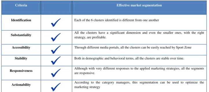
Therefore, we decided to evaluate this segmentation (Table 9) using several criteria to see

the adequacy and consistency of these segments (Clusters):

Table 9 – Segmentation validation

Criteria Effective market segmentation

Identification Each of the 6 clusters identified is different from one another

Substantiality All the clusters have a significant dimension and even the smaller ones, with the right strategy, are profitable.

Accessibility Through different media portals, all the clusters can be easily reached by Sport Zone

Stability Both in demographic and behavioral terms, all the clusters are stable over time.

Responsiveness Although with very different responses to the applied marketing strategies, all the segments are responsive.

(24)

22

17. Limitations and Future Research

Our main limitations are centered in the misallocation of some stores due to some variables

limitations (more specifically “income and “competition”). Via Catarina and Spacio Olivais

both use the income of Porto and Lisbon, respectively, and are both located in one of the

poorest parts of both cities. After comparing both of their data, we concluded that the best

possible strategy is to treat them together in terms of marketing strategy.

Castelo Branco and Guarda were majorly allocated to the “Average” cluster because of the

high competition. However, all the other variables are extremely close to the “Interior”

cluster. We would advise category managers to treat both of them as being part of the

“Interior” cluster but bearing in mind the high competition that both of these stores are

subjected to. At last, Rio Tinto is a very odd store and despite being allocated to the

“Islands” cluster, its data cannot be fully understood. Apart from having few youngsters,

Rio Tinto store has low “income” and low “promotions” which is a sort of paradox.

Reinforcing even more this idea is the fact that the store has High supplier brand. For all

these reasons, it is the store which absolutely needs to be treated separately.

Regarding the next steps, we think that this specialized retail store must do a proper

targeting and positioning. To do so, there must be an estimation of the profitability and

accountability of all the six segments. Moreover, the bargaining power of all the

intervenients in the business must be measured and, only afterwards, can the company

choose the best segments to target. The last part of the STP process is the positioning. This

specialized retail store must be able to pass the straight message to the client of what are

(25)

23

18. Bibliography

Baker, Michael. 2003. The Marketing Book. Oxford: Butterworth-Heinemann

Carmone F. J. Smith S. M. 1989. Multidimensional Scaling: Concepts and Application. American Marketing Association

Everitt, Brian. Landau, Sabine. Leese, Morven. Stahl, Daniel. 2011. Cluster Analysis. United Kingdom: John Wiley & Sons, Ltd

Lockshin, Lawrence. Spawton, Anthony. Macintosh, Gerrard. 1997. “Using product, brand and purchasing involvement for retail segmentation”. Journal of Retailing and

Consumer Services, Vol. 4,No. 3, pp. 171-183

Maroco, João. 2010. Análise Estatística – Com Utilização do SPSS. Lisboa. Edições Sílabo, Lda

Mendes, Armando. Cardoso, Margarida. 2006. “Clustering supermarkets: the role of experts”. Journal of Retailing and Consumer Services, 13, 231-247

Pallant, Julie. 2001. SPSS SURVIVAL MANUAL. Australia: Sr Edmundsbury Press, Ltd

Venkatesan, Rajkumar. 2007. “Cluster Analysis for Segmentation”.

(26)

24

LojaID Brand Promotions AverageTicket Temperature Rainfall Income Gender <15 15 - 19 20 - 24 25 - 29 30 - 34 35 - 39 40 - 44 45 - 49 50 - 54 55 - 59 60 - 64 65 - 69 70 - 74 >75 Competition Amplitude

L0933 53% 54% 50,00 17,0 60,5 100,85 52% 17,2% 5,1% 0,05 0,07 0,09 0,09 0,08 0,07 0,07 0,06 0,06 0,04 0,03 0,06 38,00 10,50

L0868 61% 69% 36,00 16,7 59,7 86,75 52% 12,6% 4,3% 0,05 0,05 0,06 0,07 0,07 0,07 0,07 0,07 0,07 0,06 0,06 0,14 89,00 11,60

L0928 85% 3% 76,00 14,7 102,0 71,62 50% 18,3% 6,8% 0,07 0,07 0,08 0,09 0,09 0,08 0,07 0,06 0,04 0,04 0,03 0,05 35,00 9,10

L0399 69% 17% 11,00 14,7 102,0 86,45 52% 16,6% 5,5% 0,06 0,07 0,08 0,09 0,08 0,08 0,07 0,06 0,06 0,04 0,04 0,05 1,00 9,10

L1664 13% 39% 64,00 16,7 59,7 94,99 52% 13,8% 4,7% 0,05 0,06 0,06 0,07 0,07 0,07 0,07 0,07 0,06 0,06 0,06 0,12 100,00 11,60

L0140 56% 71% 37,00 16,7 59,7 85,14 53% 12,9% 5,2% 0,05 0,05 0,06 0,06 0,07 0,07 0,07 0,07 0,06 0,06 0,06 0,13 0,00 11,60

L0172 72% 5% 53,00 15,4 75,6 87,31 52% 15,5% 5,7% 0,06 0,06 0,07 0,08 0,08 0,08 0,07 0,07 0,06 0,05 0,04 0,07 49,00 8,90

L0173 91% 62% 65,00 13,3 89,5 79,09 52% 12,2% 5,1% 0,05 0,05 0,06 0,06 0,06 0,07 0,07 0,07 0,07 0,06 0,06 0,12 52,00 14,60

L1572 20% 83% 97,00 13,6 97,5 79,41 52% 13,9% 5,6% 0,06 0,06 0,06 0,07 0,08 0,08 0,08 0,07 0,06 0,05 0,05 0,10 51,00 13,30

L1207 48% 34% 64,00 14,7 102,0 112,25 52% 16,8% 5,1% 0,05 0,07 0,08 0,10 0,09 0,08 0,07 0,06 0,06 0,04 0,03 0,06 74,00 9,10

L0480 56% 74% 94,00 16,7 59,7 101,45 53% 14,3% 4,7% 0,05 0,06 0,07 0,07 0,07 0,07 0,07 0,06 0,06 0,06 0,05 0,12 45,00 11,60

L0137 89% 19% 7,00 15,5 75,4 96,50 53% 13,0% 4,6% 0,05 0,05 0,07 0,07 0,07 0,07 0,07 0,07 0,07 0,06 0,06 0,11 96,00 10,80

L1573 99% 78% 86,00 15,4 75,6 82,57 52% 15,8% 5,8% 0,06 0,06 0,08 0,08 0,08 0,08 0,07 0,06 0,05 0,05 0,04 0,06 71,00 8,90

L0166 78% 44% 45,00 13,6 97,5 96,11 53% 15,3% 5,5% 0,06 0,06 0,08 0,08 0,07 0,07 0,07 0,06 0,06 0,05 0,05 0,09 57,00 13,30

L0199 95% 25% 56,00 12,3 63,2 96,47 52% 12,4% 4,8% 0,05 0,06 0,07 0,07 0,07 0,07 0,07 0,07 0,06 0,06 0,06 0,12 16,00 15,80

L0161 12% 2% 36,00 15,9 65,8 102,92 52% 15,2% 5,6% 0,06 0,06 0,08 0,08 0,08 0,07 0,07 0,06 0,06 0,05 0,04 0,08 26,00 9,80

L0192 10% 24% 47,00 14,7 102,0 70,52 51% 18,1% 7,0% 0,07 0,07 0,07 0,09 0,08 0,08 0,07 0,05 0,04 0,04 0,03 0,06 83,00 9,10

L0931 25% 44% 37,00 15,7 63,2 95,48 53% 5,8% 2,2% 0,02 0,04 0,04 0,03 0,04 0,03 0,08 0,08 0,08 0,10 0,14 0,23 58,00 16,00

L0197 66% 43% 77,00 14,8 122,5 93,09 53% 14,1% 5,3% 0,05 0,06 0,07 0,08 0,07 0,07 0,07 0,07 0,06 0,05 0,05 0,09 59,00 10,00

L0932 5% 42% 63,00 15,4 75,6 129,86 53% 14,4% 5,6% 0,06 0,07 0,07 0,08 0,08 0,08 0,08 0,07 0,06 0,05 0,04 0,08 12,00 8,90

L0138 1% 15% 77,00 15,4 75,6 126,68 53% 14,6% 5,4% 0,06 0,07 0,08 0,08 0,07 0,07 0,07 0,06 0,06 0,05 0,04 0,08 73,00 8,90

L0149 46% 100% 62,00 13,3 89,5 101,46 52% 14,9% 5,4% 0,05 0,06 0,07 0,08 0,08 0,08 0,07 0,06 0,05 0,05 0,04 0,09 3,00 14,60

L0152 32% 58% 83,00 14,7 102,0 112,25 52% 16,8% 5,1% 0,05 0,07 0,08 0,10 0,09 0,08 0,07 0,06 0,06 0,04 0,03 0,06 56,00 9,10

Appendix 1 – Dataset example

Appendixes

(27)

25

Appendix 3 – Correlations matrix Appendix 2 – Preliminary analysis

AverageTicket Brand Temperature Rainfall Promotions <15 15 - 19 20 - 24 25 - 29 30 - 34 35 - 39 40 - 44 45 - 49

50 – 54 55 - 59 60 - 64 65 - 69 70 -

74 >75 Gender Income Competition Amplitude

Mean 19,55 0,44 15,78 75,27 0,22 0,15 0,05 0,05 0,06 0,07 0,08 0,07 0,07 0,07 0,06 0,06 0,05 0,05 0,09 0,52 111,58 22,27 10,75 Standard

Error 0,32 0,01 0,19 2,93 0,01 0,00 0,00 0,00 0,00 0,00 0,00 0,00 0,00 0,00 0,00 0,00 0,00 0,00 0,00 0,00 4,28 4,38 0,25

Median 19,90 0,44 15,73 65,83 0,21 0,15 0,05 0,05 0,06 0,07 0,08 0,07 0,07 0,07 0,06 0,06 0,05 0,04 0,08 0,52 101,45 8,10 10,50

Mode #N/A #N/A 14,68 102,03 #N/A 0,16 0,05 0,05 0,06 0,08 0,08 0,07 0,07 0,06 0,06 0,06 0,05 0,05 0,08 0,53 216,88 1,60 9,10 Standard

Deviation 2,62 0,06 1,56 23,62 0,05 0,02 0,01 0,01 0,01 0,01 0,01 0,01 0,01 0,00 0,01 0,01 0,01 0,02 0,03 0,01 34,53 35,35 2,03

Sample

Variance 6,85 0,00 2,43 557,98 0,00 0,00 0,00 0,00 0,00 0,00 0,00 0,00 0,00 0,00 0,00 0,00 0,00 0,00 0,00 0,00 1192,51 1249,29 4,13

Kurtosis 0,41 -0,25 0,55 -0,90 0,14 6,04 7,82 13,04 7,36 11,11 7,15 3,44 9,81 0,26 15,27 3,75 7,54 18,53 7,25 1,36 3,67 10,37 1,01

Skewness -0,32 0,20 -0,40 0,53 0,20 -1,7 0,40 -2,2 -2,1 -2,4 -1,7 -0,9 -2,1 -0,3 -2,57 -0,5 1,91 3,97 1,98 0,18 1,98 2,95 0,66

Range 13,28 0,27 8,11 80,09 0,23 0,13 0,06 0,04 0,04 0,09 0,06 0,04 0,05 0,02 0,05 0,06 0,06 0,11 0,19 0,04 146,36 197,00 9,50

Minimum 12,73 0,31 10,87 42,43 0,11 0,06 0,02 0,02 0,03 0,01 0,03 0,04 0,03 0,06 0,03 0,03 0,04 0,03 0,05 0,50 70,52 0,00 6,50

Maximum 26,02 0,58 18,98 122,52 0,34 0,18 0,08 0,07 0,07 0,10 0,10 0,09 0,08 0,08 0,08 0,08 0,10 0,14 0,23 0,54 216,88 197,00 16,00

Largest(1) 26,02 0,58 18,98 122,52 0,34 0,18 0,08 0,07 0,07 0,10 0,10 0,09 0,08 0,08 0,08 0,08 0,10 0,14 0,23 0,54 216,88 197,00 16,00

Smallest(1) 12,73 0,31 10,87 42,43 0,11 0,06 0,02 0,02 0,03 0,01 0,03 0,04 0,03 0,06 0,03 0,03 0,04 0,03 0,05 0,50 70,52 0,00 6,50

Confidence

(28)

26

Appendix 4 – Category Managers Questionnaire

Objective: Our particular objective is to support category managers to better define the

product type to be displayed in the stores’ shelves by doing store clusters

Rate on a scale from 1 to 4 the following variables being 1 not relevant and 4 very important

Would you recommend any other variable to be considered?

Answer:__________________________________________________________________

Name:___________________________________________________________________ Category:________________________________________________________________

Dom

Domains

ains

Name 1 2 3 4

Cus

to

mers

Brand

Promotions

Average Ticket

G

eo

g

ra

ph

ic Temperature

Rainfall

Demo

g

ra

ph

ic Income

Gender

(29)

27

Appendix 7 – Rotated Component Matrix Rotated Component Matrix

Age intervals Component

1 2 3

<15 ,829 ,376 -,341 15-19 ,125 ,947 ,095 20-24 ,552 ,670 ,263 25-29 ,930 -,014 ,007 30-34 ,934 -,118 -,263 35-39 ,763 ,418 -,391 40-44 ,493 ,805 ,046 45-49 ,676 ,420 ,528 50-54 -,224 -,041 ,919

55-59 ,156 -,850 ,459 60-64 -,123 -,941 ,041 65-69 -,886 -,382 -,119 70-74 -,983 -,059 -,058 >75 -,886 -,390 ,059 Appendix 6– Clusters characteristics