Recessions in Portugal: The Predictive Power of
Term Structure of Interest Rates Components
Isabel Maldonado
Portucalense University REMIT GOVCOPP Porto, PortugalCarlos Pinho
University of Aveiro GOVCOPP Aveiro, PortugalAbstract—In this paper we present a study of the predictive ability of the term structure of interest rates over future recessions in Portugal. The analysis will be based on factor models in which the term structure of interest rates is determined by latent factors, corresponding to their level, slope and curvature. Simple and modified probit and logit models will be used to examine the forecasting ability of term structure in predicting economic crises (recessions). Recession periods were determined based on the methodology proposed by Bry and Boschan. Our results suggest that all term structure of interest rates components allow to predict recessions in one-year time horizons, with an increase in adjustment quality when we include an autoregressive term as the explanatory variable.
Keywords- Term structure of interest rates; Recessions; Factor models’ decomposition, Portugal
I. INTRODUCTION
Containing the term structure information on interest rates of different maturities, being the short-term interest rate related to the monetary policy and the long-term rate with the expectations of economic agents regarding the future economic activity [1], many studies attempt to extract from the term structure of interest rates information about the future behaviour of key macroeconomic variables. Indeed, simple financial indicators, such as interest rates and stock prices, have shown greater capacity in terms of predicting economic recessions than compound indices integrating some of the main indicators [2], especially when objective is the forecast beyond a quarterly period.
Traditionally, the term spread is considered to be quite useful in predicting output growth, inflation, industrial output, consumption and recessions [3]. Positive results have been found in the literature as to the predictive power of the term structure of interest rates over recessions ([4]; [5]). However, there are other ways of proving the relationship between the term structure of interest rates and economic activity, namely through the foreign spread [6], stock market return [4], interest rate differentials between countries [7], exchange rates [8] or by the estimation of the time structure of interest rates components extracted thru factor models.
Forecast using the term spread has presented good results in the literature. However, a number of studies, mainly conducted in the USA, indicate that the use of all term structure components contributes to improve the performance. Most
recently, [9] analyse the predictive ability of the term spread in the USA by implementing a series of linear and probit models, finding evidence that there is more information contained in the shape of the yield curve over economic activity than the one provided by the term spread alone. Also, the results presented in [10] indicate that the term structure slope and curvature together contain more information about future changes in economic activity than the isolated slope.
Our goal will be to evaluate the forecasting ability of all the of the term structure components in relation to the probability of occurrence of future recessions. The literature review shows that much more needs to be studied for European countries and for Portugal in terms of the term structure of interest rates components and their recession prediction ability. In addition, the date of these recessions can only be compared with the CEPR data, so we will adopt CEPR’s point of view in the estimation.
The first contribution of this paper is to explore the ability of the different term structure components, which extraction is based of multifactorial models, to predict recessions in Portugal. The term structure of interest rates illustrates the short-term and long-term interest rates offered by public debt securities, reflecting the rate of return of the different maturities. The forecast of economic growth through the behaviour of the term structure of interest rates can be done in two ways: on the one hand, seeking to predict the expected growth rate at a particular future moment or, on the other hand, trying to predict the probability of recession occurrence. In this work, we chose to develop the second. To that end, we used a non-parametric technique developed by [11], to determine recessions in Portugal on a monthly basis for the period from January 1984 to December 2012. Therefore, the second contribution of this paper is that, using the data obtained from the estimative of the term structure components and of the recession periods, we analyse their relationship in terms of predictability.
II. DATA AND METHODOLOGY
Our data sample includes public debt securities interest rates on with different maturities collected from the Portugal Central Bank for the period from January 1984 to December 2012. The data for determination the term structure components refers’ to monthly data for the yields of different maturities. Real GDP data was collected quarterly through the
OECD and is used to determine the recession periods and then converted into a monthly series using a methodology to be presented in the next section.
We begin by estimating the term structure components using the [12] model and then apply one algorithm to estimate the periods of expansion and recession. Finally, we join the previous steps using probabilistic logit and probit models to calculate the coefficients and the adjustment curves between both.
The Diebold and Li model used here is an extension of the three-factor parsimonious parametric model proposed by [13]. According to the authors, the forward curve will be given by:
e
te
tf
t(
)
1t
2t
3t t (1) This function consists of a constant plus a polynomial, an exponential decay term, being a class of approximation functions [14]. The solution for the second order differential equation is the forward approach curve with equal roots for the spot rates [15]. Thus, the yield curve corresponding to the Nelson Siegel forward rate curve is given by:
t t t e e e f t t t t t t 1 1 ) ( 1 2 3 (2) Where λt represents the rate of decrease over time and T the maturity. β1t, β2t and β3t, are parameters corresponding to the three dynamic latent factors, which, based on their respective weights, can be understood as long, medium and short-term components. In equation (2) the parameter λt is a time constant that determines the rate of exponential decay of the second and third components.While some authors prefer to use empirical proxies for these factors, we prefer a latent factors approach such as [16]. The authors support the option that this approach is based on a formal model, facilitating economic interpretations and also allowing the use of information across all maturities.
A solution to adjust the term structure of interest rates based on the Nelson and Siegel model would be to estimate the parameters β and λ using nonlinear least squares for each observation t. However, an alternative method to that proposed by [13] can also be applied, as discussed in [15], which uses a fixed default value for the parameter λt, which allows the calculation of factor weights. Using ordinary least squares regressions, we estimate the values of β for each day t. However, in selecting the appropriate value for the parameter λt, we follow [12]: we select the average rates to represent the average term rate and, recalling that the parameter λt governs the point where the weight of the factor β3t reaches the maximum, we choose the value of the parameter λt that maximizes the weight of the medium-term factor. Thus, a minimum squares regression can be performed on the interest rate data, obtaining the time series of the estimates of the parameters β and their corresponding residues.
Thus, as in [17] and [16], we assume that β's follow a first-order vector autoregressive process which allows us to set the latent factors model of the interest rate term structure in a space-state form and to use the Kalman filter to compute the
different estimates. Further details on the space-state model, comprising both the transition equation and the measurement equation, relating a set of N observed yields of zero coupon bonds of different maturities and the three latent factors, are found in [17] and [16]. The authors also assume that the shocks in the transition equation and in the measurement equation follow a white noise process and are mutually uncorrelated and that the shocks variance matrix is diagonal. This assumption means that the deviations of observed rates from those implicit in the term structure of interest rates are not correlated between maturity and time.
The reliability of the business cycle definition based on quarterly information may be insufficient to explain the influence of the term structure of interest rates components over recessions. The monthly timing of business cycles is likely to provide more accurate information on the exact turning points than the quarterly date. Moreover, since the economic situation is an important variable in empirical models, applications are designed that require knowledge about the turning points of the euro-zone business cycle on a monthly basis. Given the importance of using monthly data, and following [18], we chose to create a monthly chronology of the business cycle.
To determine the recessions, we used the non-parametric method, using the principles of [11] and the underlying orientation in the dating of business cycles followed by the NBER. The method developed by Bry and Boschan to detect maxima and breaks of economic activity uses an algorithm that allows to identify points of maximum and minimum values of an individual time series. Its use allows us to identify turning points based on the movements around the local maxima and minima values. Initially developed for application to monthly data, it was later expanded by [19] to allow the identification of turning points based on monthly and quarterly data. This algorithm allows us to identify the turning points in six steps. In a first step the outliers and extreme values are removed. The second step is based on the smoothing of the time series with a moving average and on the determination of the approximate turning points. In the third step, the smoothing of the time series is reduced and the turning points are adjusted for the new time series and the definition of the minimum duration for the cycles is also applied. In the fourth step, the smoothing is reduced again and the inflection points are readjusted. The fifth step re-sets the turning points for the original time series and again imposes a minimum duration for the cycles. In the sixth step, the turning points calculated in the previous five steps are presented. In this way, being Yt a representative series of
aggregate economic activity and , a local
maximum is obtained at time t if , where k = 1, 2, …,
K. A local break will occur at t if , with k = 1, 2, ...,
K. The parameter K is usually set at 5 months if the frequency of the series used is monthly.
Some assumptions have yet to be made. The basic criterion for defining each phase is that it should last at least 6 months and that a complete cycle must have a minimum duration of 15 months. The recession would correspond to the period between the maximum and the break such that, along with the five-month limit and other criteria, it is not allowed to frame recessions very often ([19]; [20]). According to [19], four items
are needed to provide useful information to have a cycle: the duration of the cycle and its phases, the amplitude of the cycle and its phases, any asymmetrical behaviour in the phases and movements accumulated within the phases.
In this work, we determine periods of recession for the period from January 1984 to December 2012. To achieve this goal, and given that the GDP data correspond to quarterly observations, we follow [18] who present two different procedures for transforming the series: soften the data or interpolate through the real quarterly GDP data based on an non-parametric estimate (the cubic spline). Considering the recess dates (turning points of the economic cycle), the estimates were always compared with the data provided by the CEPR in order to improve the reliability of the estimated dates. In this way, it is guaranteed to identify specific recession points at a given time for each country under consideration, assuming that each country is an individual nation within the larger group of the European Union.
The question then arises as to what kind of variable to use. In fact, the tests can be performed using two types of dependent variables: continuous variables, such as real GDP growth or industrial output, or discrete variables, as a dummy variable for recessions.
As in [4], we use a dummy as a dependent variable to define the moment of recession. In a previous study, [2] used a probit model to predict a recession with a dummy variable, Rt, which would be 1 if the economy was in recession in period t or 0 otherwise. The choice to forecast recessions rather than predicting product growth has an implicit purpose: information on the predictability and strength of recoveries and expansions as well as information on when the recession occurs will be combined and used as an adjustment measure for a product growth model. Using a dummy variable for recession makes possible to evaluate the accuracy with which one can predict the start date and the expected extent of recessions. This work also uses models in which the dependent variable is dichotomous, that is, they assume that the variable Y, with Y = 1 or Y = 0, is only the observable manifestation of an unobservable variable Y'. Also, [4] use a simple probit model and propose a quantitative measure of adjusted pseudo R2, showing that, among the variables studied, the slope of the term structure of interest rates is the most powerful recession predictor for quarter forecast. However, the authors use the spread rather than the decomposition of the term structure components proposed in this work.
To estimate the probability of a recession at a given point in time, we start with a non-linear probit model such as [21], [4], [7], among others, where:
{ (3)
were Rt is an observable recess indicator corresponding to a binary variable that indicates whether the economy is in recession or expansion, such that:
(4)
Where Yt is an unobservable variable that determines the occurrence of a recession at time t. α and β are the coefficients
to be estimated, being α constant and β a vector of coefficients. Xt is the vector of independent explanatory variables and ε is the error term. The parameter k corresponds to the dimension of the prediction.
The model to be estimated will then be: (5)
Where F corresponds to a cumulative normal distribution function such as -ε.
The simple probit model assumes independent error terms and evenly distributed around the zero mean. However, [22] states that this hypothesis is not plausible since, for time-series data, the error terms can be highly correlated. This led to the development of the modified probit model, which integrates a lagged of the dependent variable in order to remove any possible correlation in the series of errors. In this way, a lagged of the dependent variable is added as an explanatory variable, including a dynamic structure to the model. The dynamic or modified probit model is specified as follows:
(6)
Where Rt is the lagged dependent variable.
In the same sense, [7] results suggest that the addition of a
lagged dependent variable improves the prediction
performance of the probit model. In this study we also used the simple logit model and the modified logit model for robustness tests. We will conclude that the logit model does not bring additional benefits to those obtained using the probit model, only confirming the robustness of the results.
As mentioned, when comparing the adjustment quality for the nonlinear model, the standard and adjusted R2 is no longer an adequate measure. With this in mind, [4] suggest an alternative method to measure the quality of the adjustment of estimated nonlinear equations corresponding to the coefficient of determination of a standard linear regression model. This measure was known as the pseudo R2 and can be represented by: c L N c n L L log 2 2 1 R Pseudo (7)
Ln is the maximum unrestricted value of the likelihood function L and Lc the maximum value of the constrained model based on the assumption that all coefficients are zero, except for the constant term α. N is the number of observations in the model. [4] mention that this function guarantees that the values 0 and 1 correspond to zero of adjustment and to perfect adjustment, respectively. The pseudo R2 is used in conjunction with the probabilities of the estimated coefficients and Z statistics in order to determine the correct lag that produces the best model fit for all variables studied [23].
The simple and modified probit and logit models used here were estimated using the term structure of interest rates components as explanatory variables, in addition to the autoregressive variable for the modified versions, with forecast horizons ranging from 1 to 18 months. The statistical significance of the estimated coefficients is measured by the Z
statistic and by the probability statistics, in both versions of the model, in order to determine the explanatory power of the term structure of interest rates components over European recessions. The optimum forecast horizon is determined by the size of the offset that produces the highest pseudo R2. In the following section we present the estimation results.
III. RESULTS
Figures 1 present the results of the recession periods estimation for Portugal and of the term structure components in the following order: level, slope and curvature.
Note: This figure presents the recession periods identified for Portugal (grey) and the three term structure components evolution (red line). The first plot refers to the level (NS1), the second to the slope (NS2) and the third to the curvature (NS3). The data period considered goes from January 1984 to December 2012. Values in the Y axis refer to units in the case of the level and to percentage for slope and curvature.
Figure 1. Recessions evolution and term structure components estimation for Portugal
The estimated coefficients, the pseudo R2 and the estimated value of the likelihood function are presented in Tables 1 and 2, considering a simple probit estimate and a modified probit estimate and forecast periods of 1 to 18 months.
Our results remain virtually unchanged when we use the simple logit model instead of probit. The logit results are very similar to those of probit and results of one of the models only reinforces in terms of the other model's robustness. The logit model does not bring added value to the estimates is even more evident in terms of the robustness test when considering the case of the modified models, that is, including the autoregressive term. The main observable difference refers to the adjustment quality measure, which increases when the lagged recession variable is considered as an independent variable in the estimates. As such, we only present here the probit results.
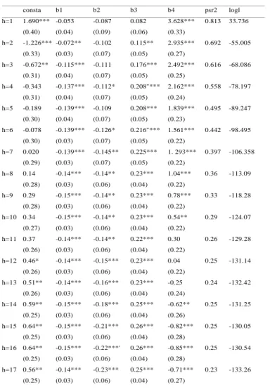
Results also prove that the inclusion of the lagged dependent variable as independent predictor greatly improves the results in terms of the adjustment quality. As such, during periods of recession the pseudo R2 increases significantly, thus
reinforcing the explanatory power of the model especially in the one month forecast horizon, thus increasing the persistence in the phases of the cycle. Also, in general terms, when the autoregressive term is included, the other explanatory variables maintain their significance, which reinforces our results. However, in some specific forecasting horizons, some of the variables lose significance, but do not lose their explanatory power, which makes them important indicators to explain recessions in Portugal.
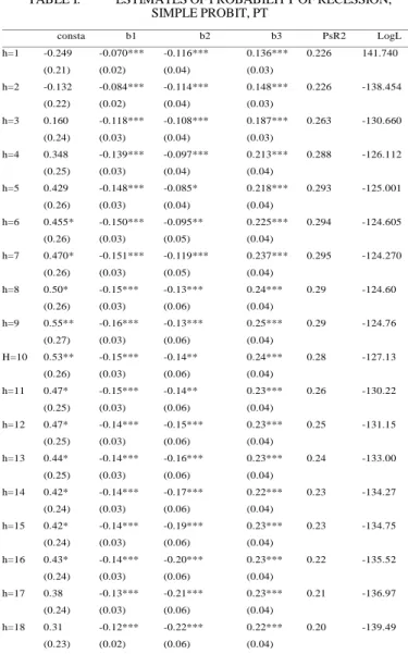
TABLE I. ESTIMATESOFPROBABILITYOFRECESSION, SIMPLEPROBIT,PT consta b1 b2 b3 PsR2 LogL h=1 -0.249 -0.070*** -0.116*** 0.136*** 0.226 141.740 (0.21) (0.02) (0.04) (0.03) h=2 -0.132 -0.084*** -0.114*** 0.148*** 0.226 -138.454 (0.22) (0.02) (0.04) (0.03) h=3 0.160 -0.118*** -0.108*** 0.187*** 0.263 -130.660 (0.24) (0.03) (0.04) (0.03) h=4 0.348 -0.139*** -0.097*** 0.213*** 0.288 -126.112 (0.25) (0.03) (0.04) (0.04) h=5 0.429 -0.148*** -0.085* 0.218*** 0.293 -125.001 (0.26) (0.03) (0.04) (0.04) h=6 0.455* -0.150*** -0.095** 0.225*** 0.294 -124.605 (0.26) (0.03) (0.05) (0.04) h=7 0.470* -0.151*** -0.119*** 0.237*** 0.295 -124.270 (0.26) (0.03) (0.05) (0.04) h=8 0.50* -0.15*** -0.13*** 0.24*** 0.29 -124.60 (0.26) (0.03) (0.06) (0.04) h=9 0.55** -0.16*** -0.13*** 0.25*** 0.29 -124.76 (0.27) (0.03) (0.06) (0.04) H=10 0.53** -0.15*** -0.14** 0.24*** 0.28 -127.13 (0.26) (0.03) (0.06) (0.04) h=11 0.47* -0.15*** -0.14** 0.23*** 0.26 -130.22 (0.25) (0.03) (0.06) (0.04) h=12 0.47* -0.14*** -0.15*** 0.23*** 0.25 -131.15 (0.25) (0.03) (0.06) (0.04) h=13 0.44* -0.14*** -0.16*** 0.23*** 0.24 -133.00 h=14 (0.25) 0.42* (0.03) -0.14*** (0.06) -0.17*** (0.04) 0.22*** 0.23 -134.27 (0.24) (0.03) (0.06) (0.04) h=15 0.42* -0.14*** -0.19*** 0.23*** 0.23 -134.75 (0.24) (0.03) (0.06) (0.04) h=16 0.43* -0.14*** -0.20*** 0.23*** 0.22 -135.52 (0.24) (0.03) (0.06) (0.04) h=17 0.38 -0.13*** -0.21*** 0.23*** 0.21 -136.97 (0.24) (0.03) (0.06) (0.04) h=18 0.31 -0.12*** -0.22*** 0.22*** 0.20 -139.49 (0.23) (0.02) (0.06) (0.04)
Notes: This table presents the coefficients estimated by the simple probit. Const refers to the constant term, b1 to the level component, b2 to slope and b3 to the curvature component of the estimated term structure. The dependent variable is a binary variable, which corresponds to 1 if there is a recession period and 0 in the other cases. PsR2 refers to the estimate of pseudo-R2, while Logl is the estimated value of the likelihood function. h represents the forecast periods ranging from 1 to 18 months. The estimated default errors are in parentheses. ***, ** and * indicate significance for the significance levels of 1, 5 and 10%, respectively. The sample observations are monthly and refer to the estimation period from January 1984 until December 2012.
Considering the simple probit model, for all forecasting horizons, all of the term structure of interest rates components have a statistically significant impact, meaning that all of them have predictive power over recessions, having as well similar
values for the adjustment quality for all the forecast horizons considered. This is justified by the characteristics of the country under consideration; Portugal was the target of a rescue of the European Union due to the recent financial crisis, which translated into deep reforms within the country in order to overcome the internal deficit.
We observe a negative impact of level and slope and the positive impact of the curvature component when we include in the probit regressions the autoregressive term. This negative sign implies that with the decrease in the level and slope of the term structure, the prospect of recession increases, which is in line with most previous studies in the literature on less developed markets such as Turkey, who consider the slope as a regressor.
However, when the autoregressive term is included, there is a positive impact on the probability of recession in Portugal but only up to 12-month forecast horizons. In addition, values of the adjustment quality increase when this additional term is included in the analysis, also decreasing when the forecast horizon increases. Nevertheless, in very short horizons the level, slope and curvature components lose some significance and the coefficient of the autoregressive term loses its significance for forecast horizons of 11, 12 and 13 months.
TABLE II. ESTIMATESOFPROBABILITYOFRECESSION, MODIFIEDPROBIT,PT consta b1 b2 b3 b4 psr2 logl h=1 1.690*** -0.053 -0.087 0.082 3.628*** 0.813 33.736 (0.40) (0.04) (0.09) (0.06) (0.33) h=2 -1.226*** -0.072** -0.102 0.115** 2.935*** 0.692 -55.005 (0.33) (0.03) (0.07) (0.05) (0.27) h=3 -0.672** -0.115*** -0.111 0.176*** 2.492*** 0.616 -68.086 (0.31) (0.04) (0.07) (0.05) (0.25) h=4 -0.343 -0.137*** -0.112* 0.208"*** 2.162*** 0.558 -78.197 (0.31) (0.04) (0.07) (0.05) (0.24) h=5 -0.189 -0.139*** -0.109 0.208*** 1.839*** 0.495 -89.247 (0.30) (0.04) (0.07) (0.05) (0.23) h=6 -0.078 -0.139*** -0.126* 0.216"*** 1.561*** 0.442 -98.495 (0.30) (0.03) (0.07) (0.05) (0.22) h=7 0.020 -0.139*** -0.145** 0.225*** 1. 293*** 0.397 -106.358 (0.29) (0.03) (0.07) (0.05) (0.22) h=8 0.14 -0.14*** -0.14** 0.23*** 1.04*** 0.36 -113.09 (0.28) (0.03) (0.06) (0.04) (0.22) h=9 0.29 -0.15*** -0.14** 0.23*** 0.78*** 0.33 -118.28 (0.28) (0.03) (0.06) (0.04) (0.22) h=10 0.34 -0.15*** -0.14** 0.23*** 0.54** 0.29 -124.07 (0.27) (0.03) (0.06) (0.04) (0.22) h=11 0.37 -0.14*** -0.14** 0.22*** 0.30 0.26 -129.28 (0.26) (0.03) (0.06) (0.04) (0.22) h=12 0.46* -0.14*** -0.15*** 0.23*** 0.04 0.25 -131.14 (0.26) (0.03) (0.06) (0.04) (0.22) h=13 0.51** -0.14*** -0.16*** 0.23*** -0.25 0.24 -132.42 (0.26) (0.03) (0.06) (0.04) (0.24) h=14 0.59** -0.15*** -0.18*** 0.25*** -0.62** 0.25 -131.25 (0.25) (0.03) (0.06) (0.04) (0.26) h=15 0.64** -0.15*** -0.21*** 0.26*** -0.82*** 0.25 -130.05 (0.25) (0.03) (0.06) (0.04) (0.28) h=16 0.64** -0.15*** -0.22***' 0.26*** -0.85*** 0.25 -130.54 (0.25) (0.03) (0.06) (0.04) (0.28) h=17 0.56** -0.14*** -0.23*** 0.25*** -0.71*** 0.23 -133.26 (0.25) (0.03) (0.06) (0.04) (0.27) h=18 0.45* -0.13*** -0.23*** 0.23*** -0.54** 0.21 -137.13 (0.24) (0.02) (0.06) (0.04) (0.25)
Notes: This table presents the coefficients estimated by the modified probit. Const refers to the constant term, b1 to the level component, b2 to slope and b3 to the curvature component of the estimated term structure. The dependent variable is a binary variable, which corresponds to 1 if there is a recession period and 0 in the other cases. PsR2 refers to the estimate of pseudo-R2, while Logl is the estimated value of the likelihood function. h represents the forecast periods ranging from 1 to 18 months. The estimated default errors are in parentheses. ***, ** and * indicate significance for the significance levels of 1, 5 and 10%, respectively. The sample observations are monthly and refer to the estimation period from January 1984 until December 2012.
Figures 2 and 3 shows the predictive power of both logit (the red line) and probit (the blue line) models estimated for the different forecast horizons, that is, 1, 3, 6, 9, 12 and 15 months. Again, we note that the use of one or the other model is indifferent. In these plots, we present the probability of a recession given by the model, that is, the adjustments of the model in both logit and probit estimates.
Figure 2. Recessions and predictive power of simple logit and probit models for forecast horizons of 1, 3, 6, 9, 12 and 15 months.
Figure 3. Recessions and predictive power of modified logit and probit models for forecast horizons of 1, 3, 6, 9, 12 and 15 months.
The results robustness reinforces the assertion that the term structure of interest rates should be considered a useful
predictor of recessions in Portugal and all term structure components can be used as a good indicator of recession. This predict ability remains unchanged when the probit model is extended to include the autoregressive term, as well as when we use the simple logit and modified logit models, including only term structure components or including term structure components and the autoregressive term.
IV. SUMMARY AND CONCLUSIONS
This paper analyses the forecasting ability of the term structure of interest rates components for Portugal, considering monthly data from interest rate public debt with different maturities.
The results indicate that the term structure of interest rates components slope and level have a significant influence over the whole period and forecast horizons considered. The positive sign of curvature indicates that when it decreases, the probability of recession also decreases. The level and the slope have a negative influence on the recession probability.
In addition, the measure of the adjustment quality improves when the autoregressive term is included. Nevertheless, this adjustment quality decreases when the forecast horizon increases, making it clear that the forecasting power of the term structure of interest rates appears to be declining over time, as other authors' results confirm.
Future research includes the application to other European countries (currently under development) as well as the inclusion of other macroeconomic aggregates to assess the forecasting ability of the term structure of interest rates.
REFERENCES
[1] Estrella, A. and Mishkin, F. (1997), The predictive power of the term structure of interest rates in Europe and the United States: Implications for the European Central Bank, European Economic Review, 41 (7), 1375-1401.
[2] Estrella, A. and Mishkin, F. (1996), The yield curve as a predictor of US recessions. Current Issues in Economics and Finance, Federal Reserve Bank of New York, 2 (7), 1-6.
[3] Wheelock, D. and Wohar, M. (2009), Can the term spread predict output growth and recessions? A survey of the literature, Federal Reserve Bank of St. Louis Review, September/October 2009, 91(5, Part 1), 419-440. [4] Estrella, A. and Mishkin, F. (1998), Predicting U.S. recessions:
Financial variables as leading indicators, Review of Economics and Statistics, 80, 45-61.
[5] Haubrich, J. and Dombrosky, A. (1996), Predicting real growth using the yield curve, Federal Reserve Bank of Cleveland Economic Review, 32, 26-35.
[6] Bernard, H. and Gerlach, S. (1998), Does the term structure predict recessions? The international evidence, International Journal of Finance and Economics, 3, 195–215.
[7] Nyberg, H. (2010), Dynamic probit models and financial variables in recession forecasting, Journal of Forecasting, 29, 215-230.
[8] Bismans, F. and Majetti, R. (2013), Forecasting recessions using financial variables: the French case, Empirical Economics, 44, 419-433. [9] Evgenidis, A. and Siriopoulos, C. (2014), Does the yield spread retain its
forecasting ability during the 2007 recession? A comparative analysis, Applied Economics Letters, 21 (12), 1-6.
[10] Argyropoulos, E. and Tzavalis, E. (2013), Forecasting economic activity from yield curve factors, Working Paper Series, Athens University of Economics and Business, 21p.
[11] Bry, G. and Boschan, C. (1971), Cyclical analysis of time series: selected procedures and computer programs, Working Paper, New York, NBER.
[12] Diebold, F. and Li, C. (2006), Forecasting the term structure of government bond yields, Journal of Econometrics, 130 (2), 337–364. [13] Nelson, C. and Siegel, A. (1987), Parsimonious modeling of Yield
curves, Journal of Business, 60 (4), 473-489.
[14] Courant, R. and Hilbert, D. (1953), Methods of mathematical physics. vol. 1. Interscience, New York, 297–306.
[15] Shaw, F., Murphy, F. and O’Brien, F. (2014), The forecasting efficiency of the dynamic Nelson Siegel model on credit default swaps, Research in International Business and Finance, 30, 348– 368.
[16] Aguiar-Conraria, L., Martins, M. and Soares, M. (2012), The yield curve and the macro-economy across time and frequencies, Journal of Economic Dynamics and Control, 36, 12, 1950-1970.
[17] Diebold, F., Rudebusch, G. and Aruoba, S. (2006), The macroeconomy and the yield curve: a dynamic latent factor approach, Journal of Econometrics, 131(1/2), 309-338.
[18] Moench, E. and Uhlig, H. (2005), Towards a monthly business cycle chronology for the Euro Area, Journal of Business Cycle Measurement and Analysis, 1, 43-69.
[19] Harding, D. and Pagan, A. (2002), Dissecting the cycle: a methodological investigation, Journal of Monetary Economics, 49, 365-381.
[20] Pagan, A. (2010), Can Turkish recession be predicted?, Tüsiad-Koç University Economic Research Forum, Working Paper Series, Working Paper nº 1027.
[21] Estrella, A. and Hardouvelis, G. (1991), The term structure as a predictor of real economic activity, Journal of Finance, 46, 555-576.
[22] Dueker, M. (1997), Strengthening the case for the yield curve as predictor of US recessions. Federal Reserve Bank of St. Louis Review, 79 (2), 41-51.
[23] Aziakpono, M. and Khomo, M. (2007), Forecasting recession in South Africa: A comparison of the yield curve and other economic indicators, South African Journal of Economics, 75 (2), 194-212.