Relationship between hand grip strength and physical activity, nutrition and body composition in healthy people vs. unhealthy people

UNIVERSIDADE TÉCNICA DE LISBOA FACULDADE DE MOTRICIDADE HUMANA

RELATIONSHIP BETWEEN HAND GRIP STRENGTH AND PHYSICAL ACTIVITY, NUTRITION AND BODY COMPOSITION IN HEALTHY PEOPLE

VS. UNHEALTHY PEOPLE

Dissertação elaborada com vista à obtenção ao grau de Mestre na

Especialidade de Exercício e Saúde

Orientador: Professor Doutor Luis Fernando Cordeiro Bettencourt Sardinha e Professor Elvis Carnero

Júri:

Presidente

Professor Doutor Luis Fernando Cordeiro Bettencourt Sardinha

Vogais

Professora Doutora Analiza Mónica Lopes Almeida Silva Professora Doutora Maria Helena Santa Clara Pombo Rodrigues

MANUEL CALVO GARCIA 2016

2 Acknowledgements

To Professor Luis B. Sardinha, for having given me the opportunity of discovering the science of exercise and health and guiding my study.

To Professor Elvis Carnero, my adviser and friend, who guided the dissertation and spent all time I needed to clarify all doubts, to organize tests and transmitting his knowledge from first time. I do not have enough words of thanks.

To Dr. Juan de Dios Benitez, for sharing equipment for testing participants. To Dr. Lorena Correas, for helping me with nutrition analyses.

To my family for letting me study in Lisbon during a difficult season and support me during last years.

To all individuals who participated on this study.

4

INDEX

3.3.1 Physical Activity Questionnaire. ... 27

3.3.2 Nutritional questionnaire (protein intake). ... 28

3.3.3 Health Questionnaire. ... 28 3.4. Blood pressure... 29 3.5. Body Composition... 30 3.6. Strength... 32 3.7. Statistical Analyses... 32 4. RESULTS ... 34 5. DISCUSSION ... 61

5.1. Nutrition and strength ... 61

5.2. Body composition and strength ... 62

5.3. Physical Activity and strength ... 64

5.4. Sarcopenic obese group and non-sarcopenic obese group ... 65

5.5. Predictors of strength from regression models... 66

5.6. Limitations ... 66

6. CONCLUSIONS ... 68

7. REFERENCES ... 69

5

RESUMO

Autor: Manuel Calvo García

Orientadores: Professor Luis Fernando Cordeiro Bettencourt Sardinha e

Professor Elvis Carnero

A perda de massa isenta de gordura (MIG) e a força muscular estão intimamente relacionadas, e estão associados com o envelhecimento. Estas reduções devem ser devidas a algumas das mais importantes razões para a diminuição da força muscular na população idosa, o qual se associa com “impairment” funcional. Estas perdas de MIG e força muscular são denominadas sarcopenia. Normalmente a perca de força de pressão manual (PM) é maior que as percas de massa muscular no envelhecimento; embora as doenças e a obesidade tem sido factores que influencia a perda de força, a sua associação com outros factores do estilo de vida tem sido pouco estudada. O objetivo deste estudo foi analisar as relações entre os determinantes clássicos de força, nutrição, actividade física (AF) e FM. Adicionalmente, comparar estes mesmos parâmetros entre grupos sem (GS) e com doenças (GNS), e com obesidade sarcopénica (GOS) e sem obesidade sarcopénica (GSOS). Também foram analisados os determinantes da FM. Métodos: Um total de 103 sujeitos (61.16±7.74 anos; 70.43±12.33 kg) participaram neste estudo transversal. A composição corporal foi avaliada com bioimpedância tetrapolar. Actividade física e ingestão nutricional foram estimadas com questionários. A FM foi avaliada usando dinamômetro manual. As associações entre variáveis foram avaliadas usando coeficientes de correlação Pearson e Spearman; as diferenças entre grupos foram analisadas utilizando Test-t para amostras independentes e/ou test de Mann-Whitney e procedimento regressão linear (stepwise) múltipla foram usados para estimar os determinantes da FM.

Resultados: O GS teve correlações positivas entre FM y AF (r = 0.286; P< 0.05), a ingestão total de proteína em gramas (r = 0.543; P< 0.01), a MIG (r = 0.852; P< 0.005), e o índice de massa isenta de gordura (IMIG) (0.748; P< 0.05). Adicionalmente, correlações negativas ajustadas pela idade foram encontradas entre actividades da casa e FM no grupo de OG (r = -0.391; P < 0.05) e no GSOS (r = -0.383; P < 0.01). Finalmente o principal predictor da FM foi a MIG, que explicou o 68.8% da variabilidade da FM.

6

Conclusões: Os nossos resultados sugerem que elevados níveis de MIG e a ingestão total de proteína em gramas e baixos níveis de massa gorda e actividade de casa são os maiores determinantes de FM em GS e GNS da população idosa ainda quando ajustamos para a idade. Palavras-chave: força, massa isenta de gordura, ingestão de proteína, sarcopenia, obesidade sarcopénica, obesidade, massa muscular, força muscular, população idosa, composição corporal, actividade física.

7

ABSTRACT

Author: Manuel Calvo García

Mentors: Luis Fernando Cordeiro Bettencourt Sardinha e Elvis Carnero

Losses of fat free mass (FFM) and muscular strength are closely related, and they are commonly associated with aging process. These reductions must be some of the most important reasons for muscular strength in elderly people, which associated with functional impairment. These FFM losses and muscular strength reduction are denominated sarcopenia. Loss of strength is greater than losses of muscle mass with aging, although disease state and obesity must play a role in this sarcopenic syndrome. It was our aim to analyze the relationship between the classical determinants of strength, such as nutrition, physical activity (PA) and body composition, and hand grip strength (HGS) in older people, additionally compare these parameters between groups with and without disease, healthy group and unhealthy group (HG vs. UHG) or sarcopenic obesity group and non sarcopenic obesity group (SOG vs. NSOG). We also explored determinants of HGS. Methods: A total of 103 subjects (61.16±7.74 years; 70.43±12.33 kg) participated in this transversal study. Body composition was assessed by tetrapolar bioimpedance. Physical activity and nutrition were estimated using questionnaires. Strength was assessed using digital hand grip dynamometer. Pearson’s and Spearman’s coefficients of correlation were used to analyze the relationship between variables. Independent sample T-test and Mann-Whitney’s non-parametric test were utilized to compare differences between groups. Finally, stepwise linear regression was carried in order to estimate the main determinants of handgrip strength.

Results: HG had positive correlation between HGS and activity score (r = 0.286; P< 0.05), total grams of protein intake (r = 0.543; P< 0.01), fat free mass (FFM) (r = 0.852; P< 0.005), fat free mass index (FFMI) (0.748; P 0.0). Negative correlation were found adjusting for age between score house and HGS in SOG (r = -0.391; P < 0.05) and in NSOG (r = -0.383; P < 0.01). The main predictor of HGS was FFM, which explain 68.8% of HGS variability.

8

In conclusion, these results suggest that high levels FFM and total grams of protein and low percentage of FM and low score of household physical activities are the major determinant of HGS in HG and UHG elderly people even adjusted for age.

Keywords: strength, fat free mass, protein intake, sarcopenia, sarcopenic obesity, muscle mass, muscle strength, elderly people, body composition, physical activity.

9

Abbreviations List

%_hc: percentage of carbohydrates %_prot: percentage of protein intake %FM: percentage of fat mass AC: arm circumference

AMA: corrected arm muscle area ASM: apendicular skeletal muscle mass BMI: body mass index

CSA: cross sectional area

CT: X-ray computed tomography

DBP: diastolic blood pressure DEXA: dual X-ray absorptiometry

FFM: fat free mass FFMI: fat free mass index FM: fat mass

FMI: fat mass index

g_prot: total grams of protein intake HG: healthy group

HGS: hand grip strength

HGSA: hand grip strength corrected by arm area HR: heart rate

MRI: magnetic resonance imaging MS: muscular strength

MU: motor unit

NSOG: non sarcopenic obese group PA: physical activity

10 Prot_I_kg: grams protein intake per kg of body weight Prot_I_kgFFM: grams protein intake per kg of fat free mass SBP: systolic blood pressure

SD: standard deviation SMM: skeletal muscle mass SO: sarcopenic obesity SOG: sarcopenic obese group TDEI: total daily energy intake UHG: unhealthy group

11

INDEX OF FIGURES

Figure 1. Theoretical determinants of strength. PA, physical activity. ... 16 Figure 2. Paradigm of theoretical mechanism of body composition influence on strength. FFM, fat free mass; FM, fat mass; PA, physical activity... 18 Figure 3. Theoretical connection between disease and muscle strength. ... 24 Figure 4. Scatter plot representing adjusted correlation by age between score house and hand grip strength. Y-axis units are residuals of hand grip strength and age regression and X-axis are residuals of score house and age regression ... 50 Figure 5. Scatter plot representing adjusted correlation by age between score house and hand grip strength (HGS) in sarcopenic obese group (SOG) and non sarcopenic obese group (NSOG). Y-axis units are residuals of HGS and age regression and X-axis are residuals of score house and age regression ... 58 Figure 6. Scatter plot representing adjusted correlation by age between score activity and hand grip strength (HGS) in sarcopenic obese group (SOG) and non sarcopenic obese group (NSOG). Y-axis units are residuals of HGS and age regression and X-axis are residuals of score activity and age regression. ... 58 Figure 7. Scatter plot between HGS (hand grip strength) and predicted values of HGS from linear regression analyses. Independent variables= fat free mass, age, sex and corrected arm muscle area. Dashed line represents adjusted regression line and solid line is identity line. ... 59 Figure 8. Scatter plot between HGS (hand grip strength) and predicted values of HGS from linear regression analyses for healthy group (HG) on the left side and for unhealthy group (UHG) on the right side. Independent variables= fat free mass, age, sex and corrected arm muscle area. Dashed line represents adjusted regression line and solid line is identity line. ... 60

12

INDEX OF TABLES

Table 1. Characteristic of the sample ... 35

Table 2. Characteristics of nutrition ... 36

Table 3A. Chi-square for male and female group, healthy and unhealthy group ... 36

Table 4. Body composition in healthy and unhealthy group ... 37

Table 5. Body composition in male and female group... 38

Table 6. Physical activity in healthy and unhealthy group ... 39

Table 7. Physical activity in male and female groups. ... 40

Table 8. Correlation between body composition and strength.. ... 41

Table 9. Correlation between strength and nutrition. ... 42

Table 10. Correlation between strength and physical activity. ... 42

Table 11. Correlations between strength and physical activity in male and female group. ... 43

Table 12. Correlations between strength and physical activity in healthy and unhealthy group. 44 Table 13. Correlation between strength and nutrition in male and female group. ... 45

Table 14. Correlation between strength and nutrition in healthy and unhealthy group. ... 45

Table 15. Correlation between body composition and strength in male and female group. ... 46

Table 16. Correlation between body composition and strength in healthy and unhealthy group ... 47

Table 17. Correlation between body composition and strength controlling for age. ... 48

Table 18. Correlation between strength and nutrition controlling for age ... 49

Table 19. Correlation between strength and physical activity after controlling for age... 50

Table 20. Correlation between body composition and strength controlling for age in male and female group. ... 51

Table 21. Correlation between body composition and strength controlling for age in healthy and unhealthy group. ... 52

Table 22. Correlation between strength and nutrition controlling for age in male and female group ... 53

Table 23. Correlation between strength and nutrition controlling for age in healthy and unhealthy group ... 54

Table 24. Correlation between strength and physical activity controlling for age in male and female group ... 54

Table 25. Correlation between strength and physical activity controlling for age in healthy and unhealthy group ... 55

Table 26. Descriptive sarcopenic obese group and non sarcopenic obese group body composition and difference between male and female group... 56

13

Table 27. Correlation between strength and body composition in sarcopenic obese group and non sarcopenic obese group... 57 Table 28. Linear regression model for hand grip strength prediction from sex, age and body composition. ... 59 Table 29. Linear regression model for hand grip strength prediction from sex, age and body composition for healthy and unhealthy group. ... 60

14

1. INTRODUCTION

Skeletal muscle mass (SMM) loss and function related with aging process represent an important public health issue, which affects mainly older people. This combination of reduced SM and strength is known as sarcopenia. SM tissue accounts for almost half of the human body mass and is a main factor in maintaining metabolic homeostasis (i.e. glucose homeostasis), muscle strength and functionality. Moreover, loss of mobility due to age-related SM deterioration is one of the primary determinants of the need for nursing home care and dependence. It has been estimated that sarcopenia costs the United States over $18 billion per year in healthcare expenses (Janssen I, Shepard DS, 2004), which could be partially reduced with lifestyle interventions. Additionally, another modifiable health risk factors as obesity have been suggested to exacerbate sarcopenia, so older sarcopenic patients could accumulate excess of adiposity independently of losing SM, which has been defined as sarcopenic obesity condition.

In this previous framework the implementation of new exercise and nutrition intervention must be a cornerstone to improve the quality of life, health and independence of elderly population. However, several mechanism and associations between SM, physical activity (PA), nutrition and disease, and strength need to be more studied. The work presented in this manuscript explores the associations between muscle strength, protein intake and PA in a sample of older adults with and without disease. Furthermore, we have tried to analyze if older adults classified as sarcopenic obese had different characteristics in strength, nutritional variables or PA in comparison with non sarcopenic obese adults.

15

2. BACKGROUND

Losses of fat free mass (FFM) and muscular strength (MS) are closely related, and they are commonly associated with the aging process (Flynn, Nolph, Baker, Martin, & Krause, 1989; Going, Williams, & Lohman, 1995). These reductions must be some of the most important reasons for muscular dysfunctions (lower muscle efficiency to develop muscular tension) in elderly people, which have been associated with functional impairment (difficulty to perform daily physical activities) (Morley, et al., 2011), diseases (Conroy, et al., 2012; Park, et al., 2009; Park, et al., 2006) and even mortality (Newman, et al., 2006). These FFM losses and MS reduction, which may happen during senescence, are denominated sarcopenia (from the Greek

roots sarx (flesh) and penia (loss) (Newman, Kupelian, et al., 2003; Rosenberg, 1989).

Sarcopenia occurs with normal aging, and it must happen at an accelerated rate in catabolic illnesses even with minimal or no weight loss (cachexia) and most rapidly of all during unintentional weight loss (wasting). Muscle strength and power decline more than muscle dimensions (Narici, et Maffulli, 2007). The term coined by Rosenberg, which is widely used to describe SM loss, is often used to describe both a set of cellular processes (denervation, mitochondrial dysfunction, inflammatory and hormonal changes) and a set of outcomes such as decreased muscle strength, decreased mobility and function, increased fatigue, increased risk of

metabolic disorders, and increased risk of falls and skeletal fractures. Since, it may responsible

for a high percentage of cases of muscular disability (Roubenoff, 2000), sarcopenia has become a major concern for public health and research from the last decades (Cesari, et al., 2012).

There is not unanimous functional definition of sarcopenia, however the most common has been proposed by Janssen et al. (2002) in a cross-sectional survey with 4504 adults aged 60 and older and is based on a SM mass index obtain by dividing apendicular skeletal muscle mass (ASM), evaluated by dual X-ray absortiometry (DEXA), by body height squared (ASM/ht2). According to this definition, individuals presenting an ASM/ht2 ratio between -1 and -2 standard desviations (SD) of the gender-specific mean value of young controls, are categorized as having

16

class I sarcopenia. Instead, individuals with an ASM/ ht2 ratio below -2 SD are categorized as having class II sarcopenia. However, this definition did not include functional factor in the definition, which must be the clinical consequence of low functionality and maybe avoid a misclassification of sarcopenia. Recently a Report of the European Working Group on Sarcopenia in Older People have proposed additional definitions where the functional capacity and strength have been included in the definition (Cruz-Jentoft AJ, et col. 2010). However, a compose of both criteria have not been validated, which may indicate the relationship between strength, SM and functionality it is not always linear, and more factors might be involved in this relationship (Figure 1).

Figure 4 1

Figure 1. Theoretical determinants of strength. PA, physical activity.

Although, low strength on older people may be due to loss muscle mass, however low muscle strength has been proven to be an independent predictor of functional capacity, institutionalization and mortality (Visser, et al., 2005; Rantanen, et al., 2000), and some studies have showed that the loss of strength is greater than loss of muscle mass with aging

Body Composition

Age

PA

17

(Vandervoort, et al., 1986; Metter, et al., 1999). Additionally, age and body fat had significant inverse associations with strength and muscle quality (Newman, et al., 2003). So, longitudinal studies have shown that fat mass (FM) increases with age and is higher among later birth cohorts peaking at about age 60-75 years (Rissanen, et al., 1988; Ding, et al., 2007), whereas SMM and strength starts to decline progressively around the age of 30 years with a more accelerated loss after the age of 60 (Rantanen, et al., 1998; Frontera, et al., 2000). Visceral fat and intramuscular fat tend to increase, while subcutaneous fat in other regions of the body declines (Beaufrère, B., Morio, 2000; Horber FF, Gruber B, Thomi F, Jensen EX, 1997). With this scenario, the loss of SM mass and the gain of body fat with aging may potentiate each other, maximizing their effects on functional limitation in older persons an increased FM may be more predictive of self-reported disability, functional limitation, and poor physical performances than a decreased SM alone (Zamboni M, Turcato E, Santana H, 1999). This may put importance in whole body composition as playing a role as a main determinant of MS and functionality (figure 2). This may confirm results from different studies indicate that sarcopenia is only an important predictor of poor physical function after consideration of the body weight or FM of the individual (Cristini, Kan, Janssen, Morley, & Rolland, 2009; GL, 2005; Jensen GL, 2002; Zamboni M, Turcato E, Santana H, 1999).

18 Figure 4 2

Ilustración 1

Figure 2. Paradigm of theoretical mechanism of body composition influence on strength. FFM, fat free mass; FM, fat mass; PA, physical activity.

Black thick lines represent genetic and/or unknown influence of body composition variables on strength (flowchart stream). Dashed thick lines represent the influence of interaction between PA and body composition variables on strength (thin dashed lines connect the levels of interaction and plausible mechanism). Grey thick lines represent the influence of interaction between age and body composition variables on strength (thin grey lines connect the levels of interaction and plausible mechanism). Dashed box and arrow shows positive influence of nutrition on strength mediated by FFM increase.

Classical studies have been focused on mechanisms, epidemiology and efficacy of interventions for explaining strength and SMM loss with aging process. The classical studies from USA as The Framingham Heart Study beginning in 1948; The Baltimore Longitudinal Study of Aging (BLS), which start in 1957 (Ferrucci, 2008; Stone & Norris, 1966); the Harvard Alumni Health Study, a prospective cohort study, where alumni of University of Harvard were observed between 1962 and 1988, have highlighted important issues related with exercise and longevity (I. M. Lee, Hsieh, & Paffenbarger, 1995). More recently, surveys have been focused specifically in body composition area and strength, so between 1997 and 1998 was carried out

19

the baseline of The Health, Aging and Body Composition Study (Health ABC study), which included a specific section aimed to elucidated associated variables with sarcopenia, so FFM, SSM and MS were analyzed in relationship with PA and nutrition (Goodpaster, et al., 2001; Newman, Haggerty, et al., 2003). In the 21st century new studies have been focusing in different aspects related with sarcopenia, hence the elderly EXERNET Spanish multicenter study is collecting data of sarcopenia and sarcopenic obesity prevalence, and related factors (Gomez-Cabello, et al., 2011).

FFM, SM and Body Composition Influence

FFM is a complex body composition compartment, which include water, bone mineral and muscular protein. All these compartments are reduced naturally from 40 years old. However, it is well known that they do not contribute equally to strength production. The tissue-organs level must be a better-fitted approach than molecular level to study the relationship between body composition and exercise performance, since the assessment of quantitative and qualitative of SMM characteristics should be more related with exercise performance than FFM. Nowadays, there is evidence that some types of muscle are associated with diseases and hospitalization risk (Cawthon, et al., 2009), and low exercise capacity and strength (Goodpaster, et al., 2001). For in instance, low-density muscle as assessed by computed tomography (CT) has been described in older type II diabetes patients (Goodpaster, et al., 2008); expanded intermuscular and intramuscular adipose tissue assessed by magnetic resonance imaging (MRI) has been also related with several metabolic disorders (Manini, et al., 2007), poor aerobic capacity and strength production (Visser, et al., 2002). So, imaging techniques offer us the possibility to estimate muscle volume (CT and MRI), muscular density (CT) and muscular architecture (ultrasound) (Thom, Morse, Birch, & Narici, 2005). In summary, all these techniques have offered us the possibility to analyze the effect of exercise training/ regular PA and strength/functional capacity. Nevertheless, these previous studies have been concerned mainly with muscle infiltration and maximal strength, and the multicomponent approach of

20

body composition have not widely explored as related with functional capacity and/or explosive strength manifestations (power, rate of force development or rapid movements). Moreover, imaging methods are expensive and time-consuming, and most of the times unviable in field settings. Bioelectrical impedance (BIA) has been validated to assess accurately distribution of fluids in vivo in older humans (Aleman-Mateo, et al., 2010; Schoeller & Kushner, 1989). Also, anthropometric models to estimate SM have been validated, and offer the possibility to assess whole and regional SM (Heymsfield, et al. 1982), which permits us to assess SM in multiple settings.

The relationships between exercise performance, losses of FFM and/or SM components and imbalanced nutrition are not completely elucidated during senescence. Moreover, the effect of exercise training and nutrition intervention on this previous relationship is not completely well understood, and it has been proposed as a new research area of body composition study, which was recently designated as functional body composition (Sardinha, 2012). Taking together organ-tissue, cellular and molecular levels of body composition can be used to develop a better approach to understand possible mechanism related with impaired functional capacity and reduced explosive MS. Specifically, intracellular and/or muscle hydration in athletes and young subjects has been recently suggested as a mechanism of impairment of rate force development and power (Silva, A. M., Fields, D. A., Heymsfield, S. B., & Sardinha, 2010, 2011; Silva, A.M., Matias, C.N., Santos, D.A., Rocha, P.M., Minderico, C.S., Sardinha, 2014). Since water losses are inherent to aging process, it can be a rational argument that interventions focused on preserve total body water and intracellular fluids would promote a positive effect on strength (mainly power and explosive). BIA can be used to provide functional body composition mechanisms related with FFM/SM changes after exercise training programs with elders. Additionally, anthropometry offers the possibility to assess regional SM and so a better explanation of low strength performance in specific test (for in instance handgrip strength test and arm muscle area).

21 Nutrition

Nutrition is another explicative mechanism related with SM loss. So, a poor nutritional status has been reported in longitudinal observations in elders (Flynn, Nolph, Baker, & Krause, 1992). Accordingly, nutrition has been widely associated with changes of FFM and SM, so elders with higher protein intake and positive energy balances could maintain their FFM (Houston, et al., 2008); also, low micronutrient consumption was related with mobility limitation and disability (Houston, et al., 2013). In addition to inadequate nutrient intake, reduced PA is known to increase the risk of developing sarcopenia (Smith, 2014). Also, a vegetarian diet was associated with a lower SMM index than an omnivorous diet at the same protein intake (Aubertin-Leheudre, et Adlercreutz, 2009). However, reduction of protein intake was not always observed when large samples of older adults were followed over decades (Hallfrisch, Muller, Drinkwater, Tobin, & Andres, 1990), so reduced protein intake must not be the main reason for FFM reduction on elderly population in epidemiological studies. Nevertheless, most of the times a reduced daily energy intake, which is prescribed in order to reduce the excess of FM, can promote non-desirable consequences as reduction of SM, so a combined strategy of exercise training and balanced diet must be an optimized solution (Chomentowski, et al., 2009).

Exercise training and sedentary time

Exercise training and PA have strong anabolic (Chomentowski, et al., 2009; Harber, et al., 2012; Wroblewski, Amati, Smiley, Goodpaster, & Wright, 2011) and functional (Simonsick, et al., 2001) effects in older people, which can promote an increase or maintenance of SM, mainly among who practice exercises with additional resistances (Figueroa, et al., 2003; Figueroa, Park, Seo, Sanchez-Gonzalez, & Baek, 2011; Hurley, Hanson, & Sheaff, 2011; Mero, et al., 2013). Hence it has been hypothesized that elderly people involved in exercise training can maintain their SM or FFM better than others sedentary or with a low level of PA. However, maintenance of SM or FFM does not ensure completely fatigue attenuation (Katsiaras, et al., 2005), strength preservation (Delmonico, et al., 2009; Goodpaster, et al., 2001), or functional

22

capacity (Ko, Stenholm, Metter, & Ferrucci, 2012). So, it seems that some FFM components and characteristics of SM must be more important than FFM or SM alone (Delmonico, et al., 2009).

Sedentary life-style must be an important risk factor for weight gain (LaMonte MJ, 2006). Obese persons also tend to be less physically active and this may contribute to decreased muscle strength (Duvigneaud N, Matton L, Wijndaele K, 2008). Reduced PA levels described on elderly subjects have been proposed as one of the most important reasons of sarcopenia (Roubenoff, 2000; Talbot, Morrell, Fleg, & Metter, 2007), attenuate fatty acid oxidation in the muscle creating adipose tissue accumulation (Manini, et al., 2007) and its associated-strength loss and mobility (Misner, Massey, Bemben, Going, & Patrick, 1992), which can trade other disabilities (Conroy, et al., 2012; Roubenoff, 2008). Finally, muscle atrophy leads to reduction in metabolic rate both at rest and during PA and may further aggravate the sedentary state, all of which can cause increased adiposity and more SM loss.

Sarcopenic Obesity

Research has previously focused separately on the roles of obesity and sarcopenia in physical functioning and disability. As induced from figure 2, the concurrence of sarcopenia and obesity, which is known as Sarcopenic-Obesity (SO), has been reported to be a much more pejorative condition of the development of physical disabilities than either sarcopenia or obesity alone (Baumgartner RN, Wayne SJ, Waters DL & Gallagher D, 2004). Previous studies have

shown the relationships between obesity, sarcopenia and SO, although there are not much

studies, which examine the association between sarcopenic-obesity and physical function among older persons.

A cross-sectional evaluation examined the relationship between FFM and physical functioning in three groups of older adults: obese, non-obese frail, and non-obese non-frail (Villareal DT, Banks M, Siener C, Sinacore DR, 2004). The results revealed that the average FFM in the lower extremities of the obese group was significantly higher (8.5 ± 4.0 kg; mean ± SD) compared to their non-obese frail (7.0 ± 2.5 kg) and nonobese non-frail (6.5 ± 2.0 kg)

23

counterparts (Villareal DT, Banks M, Siener C, Sinacore DR, 2004). Despite having a higher absolute quantity of FFM, the percentage of body weight as FFM and muscle quality (force per unit of cross-sectional muscle area) was lower in the obese adults (Villareal DT, Banks M, Siener C, Sinacore DR, 2004). Furthermore, the obese group had scores that were equal to or lower than those of the non-obese nonfrail group in the physical performance test, peak aerobic power, and the functional status questionnaire. Similar impairments were seen in strength, walking speed, balance, and health-related quality of life (Villareal DT, Banks M, Siener C, Sinacore DR, 2004). Overweight older adults (BMI 25–30 kg/m2) are thought to be protected from disability as a lower body mass index is often associated with disability (Al Snih S, Ottenbacher KJ, Markides KS, Kuo YF & JS., 2004).

Another observational survey, with 36 women with SO, obesity was associated with

having difficulty with physical function either on its own or in the presence of sarcopenia, but sarcopenia was only associated with having difficulty with physical function in the presence of obesity but sarcopenia was not associated with difficulty in physical function in the nonobese but tended to add difficulties in the obese (Cristini et al., 2009). So, this evidence suggest that higher amounts of body fat are more associated with poor physical performance, functional limitation, and subsequent disability than is low SMM (GL, 2005; Jensen GL, 2002; Zamboni M, Turcato E, Santana H, 1999) where excess accumulation of fatty acids around the muscle fibers may interfere with their functioning (Corcoran MP, Lamon-Fava S, 2007). There are only few studies about the combined effect of obesity and muscle impairment where muscle impairment was defined by poor muscle strength. In the cross-sectional Finnish Health 2000 Survey, persons with combination of increased fat percentage and decreased muscle strength had higher prevalence of walking limitation compared to those with only high fat percentage or low muscle strength (Stenholm, et al., 2008).

Finally, Baumgartner et al. (Baumgartner RN, Wayne SJ, Waters DL & Gallagher D, 2004) reported that men with sarcopenic obesity had an odds ratio of 8.72 for two or more self-reported physical disabilities with Instrumental Activities of Daily Living, compared to 3.78 for sarcopenia and 1.34 for obesity and sarcopenic obese women had corresponding odds ratios of

24

11.98, 2.96, and 2.15, respectively (Baumgartner RN, Wayne SJ, Waters DL & Gallagher D, 2004). These results were confirmed in two later studies, where weight loss intervention combining diet and exercise among older obese people improves muscle strength and muscle quality in addition to fat loss confirming the hypothesis about tight connection between adiposity and impaired muscle function (Frimel TN, Sinacore DR, 2008; Wang X, Miller GD, Messier SP, 2007).

These findings suggest that older adults with SO have more physical frailty than older adults who suffer only of sarcopenia or obesity.

The analysis of the literature demonstrated that obese older adults exhibit physical frailty and underscore the need for an intervention to improve physical function in this population. It is reasonable to hypothesize that low muscle strength and obesity may be pathophysiologically connected which makes them more likely to be associated than expected by chance alone (figure 3).

Figure 4 3

Ilustración 2

25

Prospective cohort studies have analyzed the association of age-related loss of muscle strength and mass with adverse clinical outcomes in the older adults, including several disease or impairment conditions (Moreland JD, Richardson JA, Goldsmith CH, 2004; Nevitt MC, Cummings SR, Kidd S, 1989; Visser M, Kritchevsky S, Goodpaster B, Newman A & Stamm E,

2002). However, there is a lack of studies where the influence of disease on strength has been

analyzed in relationship with PA, nutrition and body composition. Additionally, studies covering the topic of SO and these latter variables in older people are scant in the literature.

2.1. General Objectives:

 To analyze the associations between variables of nutrition, body composition and PA with hand grip strength (HGS) variables in healthy and unhealthy groups.

 To analyze the differences on body composition, PA, nutrition and HGS between sarcopenic obese participants and non sarcopenic obese participants.

26

3. METHODS

3.1. Study Design.

This is a cross-sectional, descriptive, comparative and correlational study. It consisted in identifying the relationship between the classical determinants of strength, such as nutrition, PA and body composition, and HGS in older people.

All procedures were performed during the same day and lasted 1-hour approximately. Body composition was the first assessment, then strength and the last ones were the questionnaires. Additionally, they brought the list of medicines that they were taking. The Helsinki declaration procedures for human being studies were followed in all procedures (Kong & West, 2008).

3.2. Sample.

Our sample included 103 participants older than 50 years old, with or without chronic diseases, who take or do not take any medications that can influence fluid distribution (in instance, diuretics). They were 48 males and 55 females between 50 and 84 years-old, either sedentary or active.

The tests were carried out in the Exercise and Health Laboratory of Faculty of Human Kinetics, Mega Craque Health Club in Lisbon and Aquazul Health Club in Córdoba.

The inclusion criteria in order to participate in the study were to be at least 50 years old, be able to perform physical fitness tests and have intellectual capacity to describe their PA and nutritional habits. Before doing the assessments and filling out the questionnaire, the objective and procedure of the study was explained to each participant and an informed consent was obtained.

27

3.3. Questionnaires.

3.3.1 Physical Activity Questionnaire.

The questionnaires were filled out at the same place where the tests were done. After handing out the questionnaires, a detailed explanation was given in order to fill the questionnaires out correctly and by this obtain reliable, valid answers and one-hundred percent of compliance, on average it took twenty minutes to conclude all procedure.

The Physical Activity Questionnaire for the elderly people (Laura E. Voorrips, Anita C.J. Ravelli, Petra C.A. Dongelmans, 1991), annex 1)) was used to measure the level of PA, using 3 different categories: household activities, sport activities and leisure time activities. In the questionnaire, the participants were asked to report their habitual physical activities during the last year. Items on household activities were questions with four to five possible ratting, ranging from every active to inactive. For sports and leisure activities were asked the type of activity, hours per week spent on it, and period of the year in which the activity is usually performed. All activities were classified according to work posture and movements. An intensity code based on net energetic costs of activities, was used to classify each activity (Bink, B., F.H. Bonjer, 1966). Equations to obtain the final score were:

Questionnaire score= household score+ sport score+ leisure time activity score. Equation 4

Household score= (Q1+Q2+…+Q10)/10 Equation 5

Equation 6 Equation 7

Where Q was question, ia was intensity of sport (code), ib was hours per week of sport (code), ic was period of the year of sport (code), ja was intensity of leisure time (code), jb was hours per week of leisure time (code) and jc was period of the year of leisure time (code).

28

3.3.2 Nutritional questionnaire (protein intake).

Nutrition was assessed using the classical food records, where all macro and some micronutrients were obtained from specific software adapted to nutritional behavior of Spain and Portugal citizenships. The Portuguese intakes were calculated by nutritional frequency questionnaire of the Nutritional Epidemiology Department from the Faculty of Medicine of Porto, in annex 3, using website http://higiene.med.up.pt/freq.php. Nutritional frequency questionnaire from the Epidemiology and public Health Department from the University of Navarra, annex 4, was used for Spanish subjects. Both questionnaires were previously validated (Martin-Moreno et al., 1993).

Participants were provided with a food scale and instructed on how to complete the questionnaire. In summary, they needed to report frequency of pattern intake during the last 6-month for common serving sizes of food per 6-month, week or day.

Nutritional questionnaires gave us percentage of protein intake (%_prot). We calculated total grams of protein intake (g_prot), grams of protein intake per kg of body weight (Prot_I_kg) and grams of protein intake per kg of fat free mass (Prot_I_kgFFM).

3.3.3 Health Questionnaire.

An ad hoc previously designed health questionnaire, in annex 1, was used to know whether subjects suffer from some chronic disease, such as diabetes, heart disease, pulmonary disease or metabolic disease. Joint injury was measured using a scale from no pain to limit pain. The questionnaire asked also about medication.

Participants were categorized as healthy when without any disease, or unhealthy, who suffer from at least a disease. On the other hand, individuals were divided in sarcopenic obese group (SOG), or non-sarcopenic obese group (NSOB). Sarcopenia was defined following the HGS cut-offs by BMI category as suggested by the European Working Group on Sarcopenia in Older People (Cruz-Jentoft AJ, et col. 2010) and based on the quartiles of Fried et col. (2001) as follow:

29  Men: o If BMI was ≤ 24 kg/m2 and HGS was ≤ 29 kg o If BMI 24.1–26 kg/m2 and HGS was ≤ 30 kg o If BMI 26.1–28 kg/m2 and HGS was ≤ 30 kg o If BMI > 28 kg/m2 and HGS was ≤ 32 kg  Women: o If BMI ≤ 23 kg/m2 and HGS was ≤ 17 kg o If BMI 23.1–26 kg/m2 and HGS was ≤ 17.3 kg o If BMI 26.1–29 kg/m2 and HGS was ≤ 18 kg o If BMI > 29 kg/m2 and HGS was ≤ 21 kg

Obesity was defined according to the World Health Organization (WHO, 2000), as BMI ≥ 30 kg/m2

and/or central obesity as a waist circumference greater than 102 cm in men and 88 cm in women. When obesity, defined by BMI and/or waist circumference, and sarcopenia were presented, the participant was classified as SOG.

3.4. Blood pressure.

Blood pressure was assessed with a validated automated digital device (Omron HEM 780E) after questionnaires were filled out.

30

3.5. Body Composition.

Body composition was assessed using anthropometry and bioimpedance analysis (BIA). All procedures followed the next protocol: The last ingestion of food and liquids was 3 hours before doing the measurements; participants refrained from taking tea, coffee, chocolate or any other kind of stimulants, also they did not perform any intense exercises or efforts during the previous 24 hours.

Anthropometry. The height and weight were measured to the nearest 0.1 cm and 0.1 kg respectively with a stadiometer (Seca, Hamburg, Germany) and scale (Tanita BF510, Japan). An inextensible tape (Rosscraft, Canada) was used to obtain waist circumference (WC) and arm circumference to the nearest 0.1 cm. Triceps skinfold was measured with a calibrated caliper (Lange, USA) with 0.1 mm of precision. All measurements were carried out according to the standardized procedures described in the literature (Lohman, T. G., Roche A. F., Martorell, 1988). BMI was calculated using the Quetelet’s formula (weight (kg) / squared height (m2)).

Bioimpedance Analysis. The percentage of fat mass (%FM) was obtained by single frequency tetrapolar bioimpedance following the procedures of the manufacture (Tanita BF510, Japan, image 1). Briefly, the participants, without shoes in light indoor clothes, stood erect and still over the scale by stepping the feet electrodes. Shoulders were flexed 90º and elbows extended 180º while grapping hand electrodes. They were in this latter position until the device displayed the body composition values.

31

Image 1. Body composition analyzer tetrapolar monofrequency bioimpedance Tanita BF510

Muscle mass. Regional SMM (arm) was estimated by anthropometry. We used corrected arm muscle area (AMA) estimation since it has been classically accepted and practical in clinical settings (Gurney JM, 1973; Jelliffe EPF, 1969) . The AMA was calculated after measuring triceps skinfold thickness (TSF), and mid-arm circumference (MAC). These measurements were introduced in the mathematical model suggested by Heymsfield (1982), which was based on the following four practical approximations:

a) the mid-arm is circular;

b) the TSF is twice the average fat rim diameter; c) the mid-arm muscle compartment is circular;

d) and bone, which is included in anthropometric AMA, atrophies in proportion to muscle in protein energy malnutrition. With this procedure, AMA was overestimated between 20 to 25% due to subcutaneous fat, the medial neurovascular sheath and bone.

32 From women, corrected AMA is:

Equation 1

From men, corrected AMA is:

Equation 2

3.6. Strength.

Handgrip strength (HGS) was measured using a digital hand grip dynamometer (T.K.K.5401, Takei, Japan), which records the maximum reading in kg using the right hand. After adapting handgrip to each subject, participant stand with the right elbow extended along the body without touching the trunk or thigh with the upper limb or dynamometer, respectively. When indicated the participant squeezed the dynamometer as strong as possible during 5 seconds. Two trials were permitted with a rest period of 3 minutes and the maximal measurement was recorded. Additionally a ratio of HGS and AMA was calculated as follow (equation 3):

Equation 3

3.7. Statistical Analyses.

Statistical analysis was performed using PASW Statistics for Windows version 18.0, 2010 (SPSS Inc., an IBM Company, Chicago IL, USA). Descriptive analysis included means, standard deviation, maximum and minimum. Ranks and medians were used when variables were not normally distributed. Normality test Kolmogorov-Smirnov was used to analyze normal distribution of variables.

33

We expected to detect correlation coefficients as low as 0.25, which assuming a type I error of 0.001 and 80% of statistical power can be found with a sample size of 95 individuals.

Additionally, if we want to detect a R2 = 0.15 in a regression model with 5 independent predictor variables, a type I error of 0.05 and 80% of statistical power, we will need a minimum sample size of 91. We could recruit 103 participants, which allowed us enough statistical power to carry out the main statistical procedures in a reliable way.

Independent sample T-test and Mann-Whitney test were used to compare differences between groups (sex, SOG, NSOG, HG or UHG), for normal and non-normal distribution respectively.

Pearson’s coefficient correlation was used to analyze the associations between strength variables and independent variables. Spearman correlation coefficient was utilized when non normal distribution was detected. These previous correlations were conducted for the total sample and for unhealthy and healthy groups adjusted for age and in the same way for SOG and NSOG. Graphical representation of this partial correlations were performed by computing the residual of the regression between age and dependent variables, and on the other hand by computing residual from the regression between independent variables and age, both residuals were plotted in order to examine graphically the association between variables adjusted for age.

Stepwise linear regression analysis was used to estimate significant predictors of HGS using nutrition, body composition and PA variables as independent variables.

34

4. RESULTS

Descriptive characteristics are showed in table 1. Our volunteers were overweight on average, although some of them were close to the low weight as verified by the minimum value (19.6 kg/m2), which can be confirmed from the %FM data with range between 15.2% and 50.7%. Additionally, these participants were centrally obese as described by a mean WC of 95.8 cm. Blood pressure statistics indicated there were a wide range of healthy profiles, due to a low number of cases of hypertension (16, table 1). Regarding PA Score our questionnaire informed of low levels of total daily PA. Means of HGS and HGSA were 73.8 kg and 0.8 kg/cm2, respectively. Finally, we have got well balance sex (chi-squared=24.61, p>0.005; table 3A), also the healthy group had lower probability of not getting medication than the unhealthy group (chi-squared=22.22, p<0.005; table 3B)

35 Table 1. Characteristic of the sampleTabla 1

SD, Standard Deviation; Min, minimum; Max, maximum; Sig, statistical significant; FM, fat mass; FFM, fat free mass; BMI, body mass index; FFMI, fat free mass index; FMI, fat mass index; WC, waist circumference; SBP, systolic blood pressure; DBP, diastolic blood pressure; HGS, hand grip strength; HGSA, hand grip strength corrected by arm area; HR, heart rate; PAQ-O_Score, physical activity questionnaire for older people.

1, Kolmogorov-Smirnov test for normality distribution. *, It indicates normality distribution

Nutrition descriptive is showed in table 2. Means of total daily energy intake (TDEI) is 2113 kcal/day, total protein grams is 112.0 g and percentage of protein is 21.2% of the TDEI.

Mean SD Min Max _Sig.1

Age (years) _{61.16 ± 7.74 50.00 84.00} -Sex (M/F) -Height (cm) 164.12 ± 8.74 143.50 190.00 -Weight (kg) 70.43 ± 12.33 48.10 116.00 -% FM (%) 31.30 ± 9.29 15.20 50.70 * FFM (kg) _{48.29 ± 10.27 33.65 80.85} -BMI _(kg/m2 ) 26.09 ± 3.61 19.64 37.55 -FFMI _(kg/m2 ) 17.76 ± 2.46 12.71 24.33 * FMI _(kg/m2 ) 8.33 ± 3.24 3.20 18.00 -WC (cm) _{95.75 ± 11.32 70.00 135.00} -SBP (mmHg) 129.6 ± 19.1 80.0 176.0 -DBP (mmHg) 73.8 ± 10.0 49.0 105.0 * HGS (kg) 73.8 ± 10.0 49.0 105.0 -HGSA _(kg/cm2 ) .8 ± .3 .3 1.7 -HR (bpm) 69.2 ± 9.9 45.0 99.0 * PAQ-O_Score 7.00 ± 4.86 .00 17.68 -Hipertension (Yes/No) -Smoke (Yes/No) -Disease (Yes/No) (69/34) -Variables (16/87) (16/87) 48/55

36 Table 2. Characteristics of nutritionTabla 2

SD, Standard Deviation; Min, minimum; Max, maximum; Sig, statistical significant; TDEI, total daily energy intake; %_prot, percentage of protein; %_ch, percentage of carbohydrates; %_fat, percentage of fat; Prot_I_kg, protein intake per kg of body weight; Prot_I_kgFFM, protein intake per kg of fat free mass; g_prot, total protein grams.

1, Kolmogorov-Smirnov test for normality distribution. *, It indicates normality distribution

Table 3A. Chi-square for male and female group, healthy and unhealthy group Tabla 3

Chi-squared=24.609,

p>0.005

Table 3B. Chi-square for medication and non-medication group and healthy and unhealthy group

Chi-squared=22.222

p<0.005

Human body composition in healthy (n=34) and unhealthy (n=69) groups is shown in table 4. On average, weight was lower in the healthy (65.4 kg) than the unhealthy group (72.9 kg), as %FM was 24.7% and 34.6%, respectively. Unhealthy group (UHG) was overweight on average (27.3 kg/m2) and healthy group (HG) (25.2 kg/m2) was a normal BMI. Although healthy group had the lowest arm muscle area (42.7cm2), they performed the highest value of strength per area (0.88kg/cm2).

Mean SD Min Max Sig.1

TDEI (kcal/day) 2113.4 ± 867.9 583.0 4024.0 -%_prot _(%) 21.2 ± 4.2 14.0 32.5 -%_ch _(%) 50.7 ± 9.8 29.0 73.0 -%_fat _(%) 28.1 ± 8.8 2.0 45.0 -Prot_I_kg _{(gr/d/kg) 1.5 ± .6 .4 3.5} -Prot_I_kgFFM (gr/d/kgFFM) 2.3 ± 1.0 .6 4.7 -gr_prot (gr) 112.0 ± 53.3 27.4 260.9 -Variables

Variables Healthy Unhealthy

(n=34) (n=69)

Male 21 27

Female 13 42

Variables Healthy Unhealthy

(n=34) (n=69)

No_medica 30 27

37 Table 4. Body composition in healthy and unhealthy groupTabla 4

SD, Standard Deviation; Min, minimum; Max, maximum; Sig, statistical significant; % FM, percentage of fat mass; BMI, body mass index; WC, waist circumference; AC, Arm circumference; A_Skinfold, arm skinfold; AMA, arm muscle area; HGSA: hand grip strength corrected by arm area; FFM, fat free mass; FFMI, fat free mass index; FMI, fat mass index.

1, Kolmogorov-Smirnov test for normality distribution. *, It indicates normality distribution; $ Mann-Whitney 2. Difference between groups

$, It indicates significant difference Mann-Whitney test, p<0.05 $$, It indicates significant difference Mann-Whitney test, p<0.01 $$$, It indicates significant difference Mann-Whitney test, p<0.001

Mean Min Max Range _Sig.1 _{Mean Min Max Range}

Sig.1 Sig.2 Age (years) 59.24 ± 7.25 50.00 72.00 22.00 - 62.10 ± 7.48 50.00 84.00 34.00 - -Weight (kg) 65.41 ± 10.30 48.10 86.30 38.20 * 72.91 ± 12.57 52.20 116.00 63.80 - $$ % FM (%) 24.68 ± 6.81 15.70 37.30 21.60 * 34.56 ± 8.62 15.20 50.70 35.50 * +++ BMI (kg/m2) 23.72 ± 2.08 19.64 27.99 8.35 * 27.25 ± 3.65 20.51 37.55 17.04 * +++ WC (cm) 87.08 ± 7.78 70.00 102.50 32.50 - 100.02 ± 10.34 82.10 135.00 52.90 - $$$ AC (cm) 30.32 ± 3.52 25.00 40.50 15.50 - 31.93 ± 3.65 25.20 40.30 15.10 * $ A_Skindfold (mm) 20.96 ± 8.24 7.55 36.40 28.85 * 19.26 ± 6.75 5.20 37.75 32.55 * -HGS (kg) 33.98 ± 11.01 19.00 60.00 41.00 - 28.49 ± 9.97 13.00 53.00 40.00 - $ AMA (cm2) 42.71 ± 19.97 17.55 93.63 76.08 * 43.14 ± 15.63 20.32 90.27 69.95 * -HGSA (kg/cm2) .88 ± .30 .39 1.72 1.33 - .69 ± .22 .32 1.35 1.03 - $$ FFM (kg) 49.47 ± 9.87 33.65 64.40 30.75 * 47.70 ± 10.49 33.91 80.85 46.94 - -FFMI (kg) 17.89 ± 2.44 12.71 22.09 9.38 * 17.69 ± 2.47 13.17 24.33 11.16 - -FMI (kg) 5.82 ± 1.56 3.54 8.73 5.19 * 9.56 ± 3.15 3.20 18.00 14.80 * +++ (n=34) SD Variables

Healthy Group Unhealthy

(n=69)

38 Table 5. Body composition in male and female group.Tabla 5

SD, Standard Deviation; Min, minimum; Max, maximum; Sig, statistical significant; % FM, percentage of fat mass; BMI, body mass index; WC, waist circumference; AC, Arm circumference; FFM, fat free mass; FFMI, fat free mass index; FMI, fat mass index.

1, Kolmogorov-Smirnov test for normality distribution. *, It indicates normality distribution

2. Difference between groups

$, It indicates significant difference Mann-Whitney test, p<0.05 $$$, It indicates significant difference Mann-Whitney test, p<0.001

Mean Min Max Range Mean Min Max Range Sig.1 Mean Min Max Range Sig.1 Sig.2 WEIGHT (kg) 70.43 ± 12.33 48.10 116 67.90 76.55 ± 12.56 59.30 116 56.70 * 65.09 ± 9.38 48.10 94.80 46.70 - $$$ % FM (%) 31.30 ± 9.29 15.20 50.70 35.50 23.87 ± 6.04 15.20 38.70 23.50 - 37.78 ± 6.28 22.10 50.70 28.60 - $$$ BMI (kg/m2) 26.09 ± 3.61 19.64 37.55 17.91 26.38 ± 3.47 21.06 37.55 16.49 * 25.83 ± 3.75 19.64 37.03 17.39 - -WC (cm) 95.75 ± 11.32 70 135 65 97.15 ± 10.46 83.50 125 41.50 - 94.53 ± 11.99 70 135 65 - -AC (cm) 31.40 ± 3.67 25 40.50 15.50 32.39 ± 3.72 26.50 40.50 14 - 30.53 ± 3.43 25 40.10 15.10 - $ FFM _(kg/m2 ) 48.29 ± 10.27 80.85 33.65 47.20 57.75 ± 6.72 80.85 46.92 33.93 - 40.03 ± 3.31 48.73 33.65 15.08 - $$$ FFMI (kg/m2) 17.76 ± 2.46 24.33 12.71 11.63 19.92 ± 1.60 24.33 16.97 7.36 - 15.87 ± 1.18 19.03 12.71 6.33 - $$$ FMI _(kg/m2 ) 8.33 ± 3.24 18.00 3.20 14.80 6.46 ± 2.41 13.22 3.20 10.02 - 9.96 ± 3.00 18.00 4.42 13.58 - $$$ Male (n=48) SD SD Female (n=55) Variables Total Sample (n=103) SD

39

In table 5, human body composition variables were presented by gender groups. In male group, mean of weight (76.6kg), BMI (25.8kg/m2), waist circumference (97.2cm), arm circumference (32.4cm), FFM (57.6kg/m2), and FFMI (19.9 kg/m2) were higher than means of female group. In female group, means of %FM (37.8%) and FMI (9.96kg/m2) were higher.

PA variables in healthy and unhealthy group are presented in Table 6. In unhealthy group, means of HGS (28.49kg) , HGSA (0.69kg/cm2) and score of PAQ-O (6.98) are lower than means in healthy group, but mean of time sit in unhealthy group (2.48 hours) was higher than in healthy group (2.21 hours). Healthy group had the highest sport score mean (5.27). We found significant differences in HGS, HGSA and house score between healthy and unhealthy group (table 6).

Table 6. Physical activity in healthy and unhealthy groupTabla 6

SD, Standard Deviation; Min, minimum; Max, maximum; Sig, statistical significant; HGS, hand grip strength; HGSA, hand grip strength corrected by arm area; PAQ-O_Score, Physical Activity Questionnaire for older people score.

1, Kolmogorov-Smirnov test for normality distribution. *, It indicates significance for normal distribution. 2. Difference between groups

$, It indicates significant difference Mann-Whitney test, p<0.05 $$, It indicates significant difference Mann-Whitney test, p<0.01

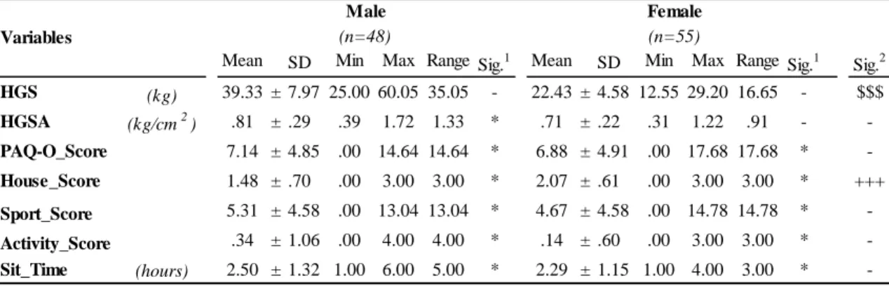
Table 7 shows male group had higher score on PAQ-O (7.14) and sport score (5.31), higher levels of HGS (39.33kg) and higher level of HGSA on average than females, although spent more time seated (table 7). Additionally, HGS in female group was lower on average (22.43kg) and range (11.65kg), they had also a significantly higher house score than men (2.07, table 7).

Mean SD Min _{Max Range Sig.}1 _{Mean SD Min Max Range Sig.}1

Sig.2 HGS (kg) 33.98 ± 11.01 19.00 60.00 41.00 - 28.49 ± 9.97 13.00 53.00 40.00 - $ HGSA (kg/cm2) .88 ± .30 .39 1.72 1.33 - .69 ± .22 .32 1.35 1.03 * $$ PAQ-O_Score 7.04 ± 4.74 .00 15.42 1.42 - 6.98 ± 4.95 .00 17.68 17.68 - -House_Score 1.56 ± .73 .00 3.00 3.00 - 1.91 ± .69 .00 3.00 3.00 - $$ Sport_Score 5.27 ± 4.56 .00 13.04 13.04 - 4.82 ± 4.60 .00 14.78 14.78 - -Activity_Score .20 ± .86 .00 4.00 4.00 - .25 ± .85 .00 4.00 4.00 - -Sit_Time (hours) 2.21 ± .98 1.00 4.00 3.00 - 2.48 ± 1.34 1.00 6.00 5.00 - -Healthy Unhealthy (n=34) (n=69) Variables

40

Table 7. Physical activity in male and female groups.Tabla 7

SD, Standard Deviation; Min, minimum; Max, maximum; Sig, statistical significant; HGS, hand grip strength; HGSA, hand grip strength corrected by arm area; PAQ-O_Score, Physical Activity Questionnaire for older people score.

1, Kolmogorov-Smirnov test for normality distribution. *, It indicates normality distribution

2. Difference between groups

+++, It indicates significant difference Test-t; p<0.001

$$$, It indicates significant difference Mann-Whitney; p<0.001

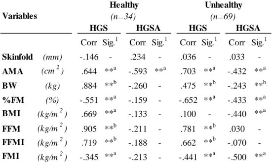
Regarding body composition and strength associations, negative Pearson’s correlation coefficients were found between arm skinfold and HGS (-0.649), %FM and HGS (-0.638), fat mass index and HGS (-0.458), arm muscle area and HGSA (-0.481), %FM and HGSA (-0.432), BMI and HGSA (-0.428) and, finally, fat mass index and HGSA (-0.488) (table 8). As expected, the relationship between muscularity and lean tissue resulted in positive Pearson’s correlation coefficients between arm muscle area and HGS (0.654), body weight and HGS (0.503); likewise the non-parametric Spearman’s correlation coefficient was positive between FFM and HGS (0.833) and fat free mass index and HGS (0.715) (table 8).

Mean SD Min _{Max Range Sig.}1 _{Mean SD Min Max Range Sig.}1

Sig.2 HGS (kg) 39.33 ± 7.97 25.00 60.05 35.05 - 22.43 ± 4.58 12.55 29.20 16.65 - $$$ HGSA (kg/cm2) .81 ± .29 .39 1.72 1.33 * .71 ± .22 .31 1.22 .91 - -PAQ-O_Score 7.14 ± 4.85 .00 14.64 14.64 * 6.88 ± 4.91 .00 17.68 17.68 * -House_Score 1.48 ± .70 .00 3.00 3.00 * 2.07 ± .61 .00 3.00 3.00 * +++ Sport_Score 5.31 ± 4.58 .00 13.04 13.04 * 4.67 ± 4.58 .00 14.78 14.78 * -Activity_Score .34 ± 1.06 .00 4.00 4.00 * .14 ± .60 .00 3.00 3.00 * -Sit_Time (hours) 2.50 ± 1.32 1.00 6.00 5.00 * 2.29 ± 1.15 1.00 4.00 3.00 * -Male Female (n=48) (n=55) Variables

41

Table 8. Correlation between body composition and strength.. Tabla 8

Corr, correlation coefficient; Sig, statistical significant; HGS, hand grip strength; HGSA, hand grip strength corrected by arm area; Skinfold, skinfold arm; AMA, arm muscle area;; PAQ-O_Score, Physical Activity Questionnaire for older people score; BW, body weight; % FM, percentage of fat mass; BMI, body mass index; FFM, fat free mass; FFMI, fat free mass index; FMI, fat mass index. *a, it indicates statistical significant Pearson’s correlation, p<0.05 ***a, it indicates statistical significant Pearson’s correlation, p<0.005 ***b, it indicates statistical significant Spearman’s correlation,

p<0.005

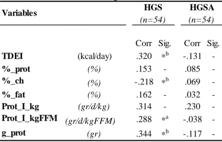
Table 9 shows correlations between strength variables and nutrition variables. Positive Spearman’s correlation coefficients were found between calories and HGS (0.320) and total protein grams and HGS (0.344), and negative coefficients between percentage of carbohydrates and HGS (-0.218, table 9). There was also a positive Pearson’s correlation coefficient between protein intake per kg of FFM and HGS (0.288, table 9).

Corr

Sig.

Corr

Sig.

Skinfold

(mm)

-.643 ***

-.124

-AMA

(cm

)

.654 ***

-.481 ***

BW

(kg)

.503

*

-.239

-%FM

(%)

-.638 ***

-.432 ***

BMI

(kg/m

)

.079

-

-.428 ***

FFM

(kg/m

)

.833 ***

-.210

-FFMI

(kg/m

)

.715 ***

-.089

-FMI

(kg/m

)

-.458 ***

-.488 ***

Variables

HGS

HGSA

(n=103)

(n=103)

42

Table 9. Correlation between strength and nutrition. Tabla 9

Corr, correlation coefficient; Sig, statistical significant; HGS, hand grip strength; HGSA, hand grip strength corrected by arm area; TDEI, total daily energy intake; %_prot, percentage of protein; %_ch, percentage of carbohydrates; %_fat, percentage of fat; Prot_I_kg, protein intake per kg of body weight; Prot_I_kgFFM, protein intake per kg of fat free mass; g_prot, total protein grams.

*a, it indicates statistical significant Pearson’s correlation, p>0.05 *b, it indicates statistical significant Spearman’s correlation, p>0.05

Correlations between strength and PA variables are showed in table 10. A negative correlation was found between house score and HGS (-0.355) and a significant and positive correlation between activity score and HGS (0.236).

Table 10. Correlation between strength and physical activity. Tabla 10

Corr, correlation coefficient; Sig, statistical significant; HGS, hand grip strength; HGSA, hand grip strength corrected by arm area Corr, correlation; Sig, statistical significant; HGS, hand grip strength; HGSA, hand grip strength corrected by arm area; PAQ-O_Score, Physical Activity Questionnaire for older people score.

*a, it indicates statistical significant Pearson’s correlation, p<0.05 ***a, it indicates statistical significant Pearson’s correlation, p<0.005

Corr Sig.

Corr Sig.

TDEI

(kcal/day)

.320

*

-.131

-%_prot

(%)

.153

-

.085

-%_ch

_(%)

_{-.218 *}

_.069

-%_fat

(%)

.162

-

.032

-Prot_I_kg

(gr/d/kg)

.314

-

.230

-Prot_I_kgFFM (gr/d/kgFFM)

.288

*

-.038

-g_prot

(gr)

.344

_*

-.117

-Variables

HGS

HGSA

(n=54)

(n=54)

Corr Sig. Corr Sig.

Sit_time _(hours) .118 - .172 -PAQ-O_Score .450 - .054 -Activity_Score .236 * -.106 -Sport_Score .063 - .039 -House_Score -.355 *** -.091 -Variables HGS HGSA (n=103) (n=103)

43

In table 11, a significant correlation was found in female group between HGS and sit time (0.311).

Table 11. Correlations between strength and physical activity in male and female group.Tabla 11

Corr, correlation coefficient; Sig, statistical significant; HGS, hand grip strength; HGSA, hand grip strength corrected by arm area; PAQ-O_Score, Physical Activity Questionnaire for older people score.

*a, it indicates statistical significant Pearson’s correlation, p<0.05

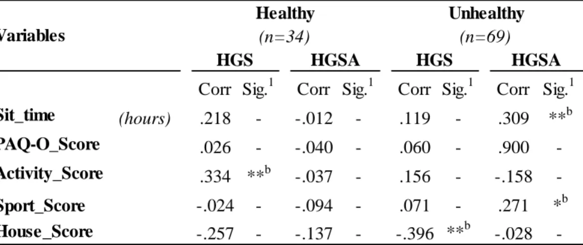
In healthy group, activity score and HGS were the only significantly associated variables (0.334) (table 12). While in unhealthy group, positive correlations were found between HGSA and sit time (0.309), HGSA and sport score (0.271) and negative correlation between house score and HGS (-0.396, table 12).

Corr Sig.

Corr Sig.

Corr Sig.

Corr Sig.

Sit_time

_(hours)

_-.123

_-

_.720

_-

_.311

_*

.259

-PAQ-O_Score

_.026

_-

_-.009

_-

_.079

_-

_.009

-Activity_Score

_.245

_-

_-.169

_-

_.199

_-

_-.640

-Sport_Score

-.019

-

.026

-

.060

-

.026

-House_Score

-.067

-

.022

-

-.009

-

-.054

-HGS

Variables

Male

Female

HGSA

HGS

HGSA

(n=48)

(n=55)

44

Table 12. Correlations between strength and physical activity in healthy and unhealthy group.Tabla 12

Corr, correlation coefficient; Sig, statistical significant; HGS, hand grip strength; HGSA, hand grip strength corrected by arm area; PAQ-O_Score, Physical Activity Questionnaire for older people score.

*b, it indicates statistical significant Spearman’s correlation, p<0.05 **b, it indicates statistical significant Spearman’s correlation, p<0.01

Table 13 shows correlations in male and female groups between strength and nutritional variables. Both females and males associations with HGS were positive, conversely HGSA was always negatively correlated.

Corr Sig.1 Corr Sig.1 Corr Sig.1 Corr Sig.1

Sit_time _{(hours) .218 - -.012 - .119 - .309 **}b PAQ-O_Score _{.026 - -.040 - .060 - .900} -Activity_Score _{.334 **}b -.037 - .156 - -.158 -Sport_Score -.024 - -.094 - .071 - .271 *b House_Score -.257 - -.137 - -.396 **b -.028 -Variables Healthy Unhealthy (n=34) (n=69) HGS HGSA HGS HGSA