Bayesian Analysis of FIAPARCH Model: An
Application to S˜
ao Paulo Stock Market
Thelma S´afadi
Federal University of Lavras, Minas Gerais, Brazil
Isabel Pereira
University of Aveiro, Aveiro, Portugal
Abstract: In this paper, we develop a Bayesian analysis of a FIA-PARCH(p,d,q) model for parameter estimation and conditional variance pre-diction. In order to study the inference problem we use the Metropolis-Hastings algorithm.This methodology is illustrated in a simulation study and it is applied to a set of observations concerning the returns of IBOVESPA values.
Key-words: Asymmetry, long memory, volatility
1
Introduction
It is well known that it is often an unrealistic situation the one which only the mean response could be changing with covariates while the vari-ance remains constant over time. This is particularly obvious in financial time series where clusters of volatility can be detected visually. Consider-ing financial time series it becomes particularly unlikely that positive and negative shocks have the same impact on volatility, leading to the volatility asymmetry concept.
However, there is no particular reason to consider the conditional variance process as a linear function of lagged squared residuals (Bollerslev, 1986) or of lagged absolute residuals (Taylor, 1986). The Asymmetric Power ARCH model, APARCH (Ding et al. (1993)) is obtained if the exponent of the residual power is different from 1 and 2. The long range dependence on conditional mean observed in financial series occurs also in the volatility or conditional variance. The integrated models whose features are similar
to unit root processes where proposed to model theses characteristics. In particular, Baillie et al (1996) proposed the Fractionally Integrated GARCH, FIGARCH(p,d,q) model in order to accommodate long memory in volatility, accordingly to the most common definition of a long memory process.
In order to allow long memory and asymmetry in volatility, Tse (1998) proposed the “Fractionally Integrated Asymmetric Power ARCH”models, FI-APARCH.
So, due to the nature of FIAPARCH model, several volatility properties such as long memory, asymmetry, leverage effect and kurtosis are well cap-tured. Despite the extreme importance of this model, it has not received much attention in the literature, specially in Bayesian context.
The proposal of this work is to extend the Bayesian analysis of the APARCH model (Silva, 2006) to a Fractionally Integrated APARCH. This paper is organized as follows. In section 2 we summarize some results pre-sented in literature. Section 3 develops APARCH and FIAPARCH mod-els. Section 4 gives the general Bayes setting for the particular FIAPARCH (1,d,1) model. In section 5 we carry on a simulation study and an appli-cation to a real set data. Finally, in section 6 we present some concluding comments.
2
Literature Review
The most common definition of long memory is the one where the auto-covariance function decays at the hypergeometric rate k2d−1 (0 < d < 0.5). Consequently, the autocovariance function of a long memory process is not absolutely summable. Series with long memory present persistence in sample autocorrelations, which means significative dependence between observations spaced by a long time period. In frequency domain the feature of d is detected by the behavior of the spectral density which tends to infinite as frequency tends to zero.
The analysis of the questions concerning the appropriate modeling of the long time dependency on conditional mean of financial series was extended to the conditional variance. This area of research leads to the formulation of the integrated GARCH process, IGARCH, by Engle e Bollerslev (1986), which has some features of the unit root processes, I(1). Therefore, the effect of the shocks on the optimal prediction of the future conditional variance leads to the convergency to a non null constant of the correspondent weights for the accumulated shocks. This implies the increase of the point previsions in a linear form with the prevision horizon.
options and future contracts could exhibit an extreme dependency on initial conditions or on actual economy state. However, according to these authors, this extreme degree of dependency seems to contradict the observed behavior. Moreover, several studies (see Crato and Lima (1994) and Ding et al. (1993)) point to strong evidence of long memory on autocorrelations of squared or absolute returns. Motivated by these facts, Baillie et al.(1996) formulated the Fractionally Integrated GARCH process, that is, FIGARCH process. The differencing parameter d introduces a different behaviour: the effect of a shock to the forecast of the future conditional variance is expected to decay at a slow hyperbolic rate. In this sense and considering FIGARCH(1,d,0) Baillie et al (1996) prove the long memory in volatility of FIGARCH models. However the statistical properties, in particular the stationarity, remain unestablished. One of the limitations of FIGARCH models concerns the symmetry of the shocks impact on volatility. Thus negative and positive shocks produce the same impact on conditional variance (or volatility). Now the majority of the applications of ARCH models are in finance where there is little proba-bility that positive and negative shocks have the same impact. Due to this fact Isler (1999) suggests using other models that could incorporate asym-metry properties and could easily estimate parameters and forecast future observations.
Several time series models, such as Exponential GARCH (EGARCH) of Nelson (1990) and Threshold ARCH (TARCH) of Zakoian (1994) were pro-posed in literature. One of the most promising models is the Asymmetric Power ARCH model, APARCH, introduced by Ding et al. (1993).
Using a Monte Carlo study, Ding et al.(1993) conclude that there is no obvious reason to assume that, for one hand the conditional variance pro-cess has to be a linear function of the squared mudei lagged residuals, as it happens on the GARCH model of Bollerslev; and, for another hand the con-ditional standard deviation process has to be a linear function of the absolute lagged residuals - see Taylor (1986). This states the importance of consider-ing models with different exponents of the residual powers. Based on these arguments Ding et al. (1993) propose a model which substantially generates ARCH class. Such model is called ARCH model with Asymmetrical Power, APARCH.
Long memory and asymmetry in volatility are exhibited on Fractionally Integrated Asymmetric Power ARCH (FIAPARCH) model, proposed by Tse (1998). An extension proposal of the univariate FIGARCH e FIAPARCH to a bivariate framework is given by Dark (2004).
Long memory in volatility has been documented across a range of equity indices: the SP500 (Ding et al, 1993; Bollerslev and Mikkelsen,1996; Ding et al, 1996; Granger and Ding, 1996; Andersen and Bollerslev, 1997; Lobato
and Savin, 1998; Liu, 2000), the NYSE ( Ding et al, 1993) the Nikkey (Ding et al, 1996).
3
APARCH and FIAPARCH Models
Ding et al.(1993) concluded there was no reason for the volatility to be a linear function of the squared residuals and introduce the APARCH(p,q) model, which allows the power δ of the heteroscedasticity equation to be estimated from the data;
ǫt= ztσt, zt ∼ N(0, 1) or zt∼ t − Student (1) σδt = ω + p X i=1 αi(|ǫt−i| − γiǫt−i)δ+ q X j=1 βjσδt−j, (2)
where ω > 0, δ ≥ 0, αi ≥ 0 and −1 < γi < 1 for i = 1, ..., p and βj ≥ 0,
for j = 1, ..., q. The model introduces a Box-Cox power transformation on the conditional standard deviation process and on the asymmetric absolute innovation.
The APARCH model allows the flexible adjustment between exponential variation with the asymmetry coefficient. For this reason this model has the ability to detect asymmetrical shocks on the volatility. Specifically if leverage effect is positive, that is γ > 0, it is verified the gear shift effect; that is, a positive value of the γi means that past negative shocks have a deeper impact
on current conditional volatility of the series, than past positive shocks, as would be expected in the analysis of financial time series.
Based on the observation that the volatility tends to change quite slowly over time, Tse (1998) modifies the FIGARCH(p,d,q) model in order to al-low for asymmetries by introducing the Frationally Integrated Asymmetric ARCH, or FIAPARCH(p,d,q).
The fractional difference is given by:
(1 − B)d = 1 − dB −d(1 − d)
2! B
2− d(1 − d)(2 − d)
3! B
3− ...., 0 < d < 1
where d is the fractional differential parameter. Long memory occurs for 0 < d < 0.5.
Lets consider in (2)
and
ξt = g(ǫt) − σtδ.
Therefore, it can be rewritten as
1 − α(B) − β(B)g(ǫt) = ω + (1 − β(B))ξt,
where α(B) =Pp
i=1αiBi and β(B) =
Pq
j=1βjBj represent lag polynomials
of p and q orders, respectively.
In order to allow that volatility shock has long memory we assume that there exists a polynomial φ(B) such that
φ(B) = (1 − α(B) − β(B)g(ǫt));
then
(1 − B)dφ(B)g(ǫt) = ω + (1 − β(B))ξt,
with 0 < d < 0.5 and the roots of φ(B) = 0 are outside the unit circle. The FIAPARCH (p,d,q) model satisfies the equation
σδ t = ω 1 − β(B) + [1 − (1 − β(B)) −1φ(B)(1 − B)d](|ǫ t| − γǫt)δ; (3)
which is strictly stationary and ergodic for 0 ≤ d ≤ 1.
It is very interesting to observe that the FIAPARCH representation nests two major classes of ARCH models: The APARCH and FIGARCH models. It must be stressed that when d = 0 the FIAPARCH model reduces to the APARCH(1,1) model and when γ = 0 and δ = 2, the process is the particular FIGARCH(1,d,1) model. Some advantages of FIAPARCH(p,d,q) models pointed out by Conrad et al (2008) are allowing:
(a) an asymmetric response of volatility to positive and negative shocks (and consequently being able to traduce the leverage effect);
(b) the data to determine the power of returns for which the predictable structure in the volatility pattern is the strongest,
(c) long-range volatility dependence (that is, are able to accommodate long memory in volatility, depending on the differencing parameter d).
Considering p = 1 and q = 1, 1−β(B) and φ(B) are polynomials of degree 1 and we let β(B) = βB and φ(B) = 1−φB, we obtain the FIAPARCH(1,d,1) model with σtδ = ω 1 − β + [1 − (1 − βB) −1(1 − φB)(1 − B)d ]g(ǫt) (4)
or equivalently, σδt = ω 1 − β + λ(B)g(ǫt), (5) where λ(B) = [1 − (1 − βB)−1(1 − φB)(1 − B)d] = ∞ X i=1 λiBi.
Bollerslev and Mikkelsen (1996) establish the sufficient conditions in order to endsure the FIGARCH (1,d,1) model to be well-defined and with positive conditional variance. These inequality constrains in the FIAPARCH(1,d,1) model are:
ω > 0, δ ≥ 0, φ ≥ 0, −1 < γ < 1, β ≥ 0 (6) and λi ≥ 0, for i = 1, ....
Note that λi ≥ 0 means
β − d ≤ φ ≤ 2 − d
3 and d(φ −
(1 − d)
2 ) ≤ β(φ − β + d). The series coefficients λi ≥ 0 can be obtained recursively, considering
λi = βλi−1+ [ (i − 1 − d) i − φ]vi−1, where vi = vi−1(i − 1 − d)/i, i = 2, ...∞ with v1 = d and λ1 = φ − β + d.
Once the λicoefficients are the same in FIGARCH and FIAPARCH
mod-els, Tse(1998) states that the effects of the past residuals on future conditional volatility has the same hiperbolic decay pointed out by Baillie et al (1996)in FIGARCH models. It can be noticed that the FIGARCH model is a case where the lag coefficients decline hyperbolically, rather than geometrically, to 0. According to this, Davidson (2004) emphasized the term ”hyperbolic memory”is preferable to distinguish FIGARCH from the geometric memory case such as GARCH.
Some properties, like strictly stationarity and ergodicity, still remain open questions. Considering FIAPARCH model, the parameter estimation and the study of estimators asymptotic properties , have not received much attention in the literature. Accordingly to Bollerslev and Wooldrigde (1992) the Quasi
Maximum Likelihood Estimation (QMLE) is generally consistent, asymptot-ically normal distributed ansd with standard errors which are valid under non-normality. Baillie et al (1996) state the same properties considering the FIGARCH model. However the impact of violations in conditional normality is unknown for FIGARCH and FIAPARCH models.
4
Bayesian Analysis of FIAPARCH Models
In this section we consider a Bayesian analysis of the parameters of the model (3). Assuming that zt∼ N(0, 1), the likelihood (L) can be expressed
as L(ǫ|θ) = n Y t=1 1 p2πσ2 t exp{− ǫ 2 t 2σ2 t }, (7)
where θ = (ω, α, γ, β, δ, d), n is the number of observations and ǫ = {ǫ1, ...., ǫn}.
An approximation of the likelihood function conditioned on the p first observations can be written as
L(ǫ|θ) α n Y t=p+1 σt−1exp{− ǫ2 t 2σ2 t }. (8)
In order to perform posterior analysis we denote the log-likelihood func-tion by £ and we assume the prior distribufunc-tion P (θ) satisfying the constrains given in (6).
Hence the posterior distribution is
P (θ|ǫ) α £(ǫ|θ)P (θ) α n Y t=p+1 σt−1exp{− ǫ2 t 2σ2 t }I(ω>0)I(α≥0)I(β≥0)I(−1<γ<1)I(0<d<0.5)I(δ≥0). (9)
Besides the inequality constrains in the priors used previously, we also have λi ≥ 0.
It should be noted that standard Gibbs sampling methods are not easy to use in FIAPARCH models. Their full conditional densities have nonstandard forms. So, we use the Metropolis-Hastings algorithm with multivariate t-Student as proposal distribution.
Samples are obtained by the algorithm as follow: according to Dellaportas et al. (2000), a sample is attained after running a chain sufficiently long, in
which the accumulated quantiles behavior corresponding to each parameter are tracked - this fits to the burn-in period. Afterwards we look at the autocorrelation function in order to choose the appropriate space between the observations to get a sample non correlated approximately. Finally the convergence of chain is analyzed by the R criterium of Gelman e Rubin (1992), Z-score test of Geweke (1992) and graphic methods.
Once the estimates of the posterior parameters are obtained, and not-ing that σδ
t only depends on parameters and observations, the evaluation of
posterior conditional variances can be obtained without further difficulties. Considering FIAPARCH(1,d,1) model we obtain:
E(σδ t|ǫt) ≈ E(ω|ǫt) 1 − E(β|ǫt) + ∞ X i=1
E(λi|ǫt)Bi(|ǫt| − E(γ|ǫt)ǫt)E(δ|ǫt), (10)
where,
E(λi|ǫt) ≈ E(β|ǫt)E(λi−1|ǫt) + [
i − 1 − E(d|ǫt)
i − E(φ|ǫt)]vi−1, and vi = vi−1(i − 1 − E(d|ǫt))/i for t = 2, ..., n.
The predictive density of ǫt+1,
P (ǫt+1|ǫ) =
Z
P (ǫt+1|θ, ǫ)P (θ|ǫ)dθ, (11)
can be used to evaluate the predictive accuracy of the model under consid-eration.
In the context of the FIAPARCH model, the steps required to estimate the k one-step-ahead predictive densities ˆP (ǫt+1|ǫ), given by
ˆ
P (ǫt+1|ǫ) =
PS
s=1P (ǫˆ t+1|ǫ, θs)
S , (12)
where t = n, n + 1, . . . , n + k − 1 are the following:
1. Generate samples θs(s = 1, . . . , S) from the joint posterior distribution
P (θ|ǫ), using Metropolis-Hastings algorithm.
2. Generate samples of size S from the conditional variances σδ
t+1, using
the samples θs (s = 1, . . . , S).
4. Estimate the predictive density, by ˆ P (ǫn+1|ǫ) = 1 S S X s=1 ˆ P (ǫn+1|θs, ǫ). (13)
Since Monte Carlo Markov chain (MCMC) methods produce observations from the joint posterior distribution P (θ|ǫ), the simulations results θs, (s =
1, . . . , S) can be used to compare the models. Therefore, according to Gelfand et al. (1992) proposal we can use,
n+k−1
Y
t=n
ˆ
P (ǫt+1|ǫ). (14)
It is chosen the model which makes greater the value of Qn+k−1
t=n P (ǫˆ t+1|ǫ).
Specificaly, to compare M1 and M2 models, Gelfand et al. (1992) propose
the following quantity, D = log Qn+k−1 t=n P (ǫˆ t+1 = ǫt+1|Ψt, θ, M1) Qn+k−1 t=n P (ǫˆ t+1 = ǫt+1|Ψt, θ, M2) ! , (15) where ǫt+1 is a realization of the stochastic process at time t + 1, Ψt is the
available information until time t, and θ is the posterior mean vector of the specified model. It is chosen the model M1 (M2) if D > 0(D < 0). Gelfand
et al. (1992) called exp(D) as Bayes pseudo-Factor.
For the FIAPARCH (p,d,q) model with ztnormal or t-Student, the
resid-uals standardized ˜ ǫt = ǫt pσ2 t
are random variables i.i.d. with normal distribution or t-Student. So one way to see if the model is appropriate is to calculate the statistical Q Lung-Box for ˜ǫt. Moreover, we can calculate the coefficients of asymmetry and kurtosis
and make a qq-plot to verify the assumption of normality.
5
Results
5.1
Simulated data
We simulated 50 samples of size 500 from the FIAPARCH model with different values for the parameters. We calculated Bayesian estimates using
the Metropolis-Hastings algorithm with multivariate t-Student as the pro-ponent distribution. Due to convergence requirements we run the sampler algorithm 155100 iterations.
For each iteration we obtained the mean, mode or median of the pos-terior distribution and considering all the 50 replications we calculated the corresponding sample means and standard deviations. We studied several combinations of parameters. The results of this simulation study, for four particular sets of parameters which illustrate well the overall behavior of the estimates, are displayed in Tables (1), (2), (3). Real values of the parameters of the simulated model are indicated in the first column.
Generally, mean and median estimates are similar and behave better than mode estimate of the parameters. A closer look at the tables reveals that there is some difficulty in estimating the value of β. Depending on the mag-nitude of the parameters the correspondent real values are underestimated or overestimated.
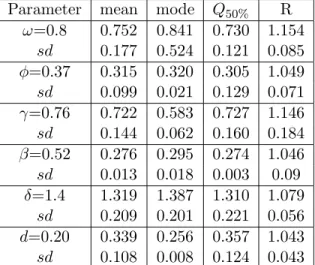
TABLE 1: Inference simulated results - gaussian model FIAPARCH(1,d,1).
Parameter mean mode Q50% R
ω=0.8 0.752 0.841 0.730 1.154 sd 0.177 0.524 0.121 0.085 φ=0.37 0.315 0.320 0.305 1.049 sd 0.099 0.021 0.129 0.071 γ=0.76 0.722 0.583 0.727 1.146 sd 0.144 0.062 0.160 0.184 β=0.52 0.276 0.295 0.274 1.046 sd 0.013 0.018 0.003 0.09 δ=1.4 1.319 1.387 1.310 1.079 sd 0.209 0.201 0.221 0.056 d=0.20 0.339 0.256 0.357 1.043 sd 0.108 0.008 0.124 0.043
Note: sd is the standard deviation, Q50% is the posterior median and R is the value of Gelman and Rubin´s criterium.
5.2
Returns of IBOVESPA data
The proposed Bayesian approach is illustrated using daily returns from S. Paulo Stock Market rates, IBOVESPA, for the period from 01/03/1994 to 30/12/2007. (www.ibovespa.com.br)
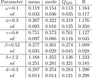
TABLE 2: Inference simulated results - gaussian model FIAPARCH(1,d,1).
Parameter mean mode Q50% R
ω=0.1 0.119 0.154 0.113 1.164 sd 0.033 0.036 0.035 0.117 φ=0.3 0.267 0.322 0.319 1.176 sd 0.095 0.016 0.135 0.350 γ=0.8 0.751 0.573 0.761 1.127 sd 0.097 0.086 0.116 0.045 β=0.52 0.277 0.301 0.274 1.089 sd 0.035 0.029 0.045 0.028 δ=1.2 1.168 1.355 1.136 1.233 sd 0.251 0.281 0.321 0.185 d=0.3 0.287 0.254 0.284 1.290 sd 0.014 0.014 0.121 0.298
Note: sd is the standard deviation, Q50% is the posterior median and R is the value of Gelman and Rubin´s criterium.
TABLE 3: Inference simulated results - gaussian model FIAPARCH(1,d,1).
Parameter mean mode Q50% R
ω=0.14 0.140 0.243 0.125 1.053 sd 0.035 0.041 0.038 0.072 φ=0.20 0.321 0.322 0.323 1.031 sd 0.038 0.008 0.053 0.029 γ=0.21 0.233 0.302 0.225 1.034 sd 0.193 0.302 0.183 0.043 β=0.38 0.267 0.366 0.253 1.034 sd 0.047 0.028 0.053 0.041 δ=1.28 1.294 1.253 1.239 1.085 sd 0.312 0.298 0.342 d=0.27 0.143 0.241 0.123 1.032 sd 0.049 0.009 0.089 0.039
Note: sd is the standard deviation, Q50% is the posterior median and R is the value of Gelman and Rubin´s criterium.
0 500 1000 1500 2000 2500 3000 3500 0 1 2 3 4 5 6 7x 10 4 IBOVESPA−01/1994−12/2007 IBOVESPA 0 500 1000 1500 2000 2500 3000 3500 −1 −0.8 −0.6 −0.4 −0.2 0 0.2 0.4 IBOVESPA return
FIGURE 1: IBOVESPA data and IBOVESPA returns.
The Figure (1) shows the IBOVESPA data and the IBOVESPA returns ǫt. The plot of autocorrelation function to ǫt ( not presented here) shows
that we need to fit a AR(10) model to the return , so we have ǫt given by
ǫt= −0.0506ǫt−4+ 0.082ǫt−10+ yt.
In the remaining of this work, the residuals yt will be denoted by
re-turns of IBOVESPA. Figure (2) shows the gaussian qq-plot to yt and the
autocorrelation functions of yt, yt2 and |yt|, respectively . Some of the
typ-ical regularities of financial time series are captured in this data set, such as: weak dependence without any evident pattern on the series level, and significative dependence on squared and absolute returns. In particular, the gaussian qq-plot presents the leptocurtosis of returns distribution. Consid-ering the long memory and the heteroscedasticity shown in Figure (2) the FIGARCH model would be indicated for fit the IBOVESPA returns. Looking at the present autocorrelation in the series y2
t and |yt| is prudent
consider-ing a model whose power of volatility could be any positive value. So, the FIAPARCH model can be useful to fit the IBOVESPA returns.
Moreover, Figure (2) shows a significative correlation on observations with large delay, so the binomial term (1 − B)d will be truncated in M=100
−2 0 2 −10 0 10 20 30 0 5 10 15 20 25 30 35 0.0 0.2 0.4 0.6 0.8 1.0 Lag y 0 50 100 150 200 0.0 0.2 0.4 0.6 0.8 1.0 Lag y^2 0 50 100 150 200 0.0 0.2 0.4 0.6 0.8 1.0 Lag |y|
FIGURE 2: Gaussian qq-plot and acf for yt, yt2 and |yt|, respectively.
For the t-Student distribution (ν, µ, Σ) used in Metropolis-Hastings algo-rithm we consider ν = 6,
µ = (0.1922, 0.0396, 0.7659, 0.8545, 0.3000, 1.6513)′ and
Σ = 0.8diag(0.0259, 0.0229, 0.2289, 0.0188, 0.012, 0.1116),
where the 0.8 multiplicative constant was chosen by empirical work in order to achieve a greater acceptance rate of Metropolis-Hastings algorithm.
To calculate the Bayesian estimates we run 400,000 iterations, among these we discarded the first 30% as burn-in time. To reduce autocorrela-tion between MCMC samples we considered only samples from every 250 iterations. Consequently we use 14,400 samples for posterior inference.
Table (4) provides numerical results for the parameter estimates. Note that the posterior means of γ and d take the values 0.6346 and 0.3331, respec-tively; these results show that past negative shocks have a deeper impact on current conditional volatility of the series as also the presence of long mem-ory in IBOVESPA series returns. It is worth to mention that the simulation study presented in previous section contains the particular set of parameters, obtained by the means of the posterior distribution, as the true values of model parameters.
TABLE 4: Inference results - gaussian model FIAPARCH(1,d,1) - returns of Ibovespa.
Parameter mean mode Q50% MC L.B U.B z-score R
ω 0.4915 0.4800 0.4740 0.011 0.3785 0.7311 0.9584 1.0523 sd 0.0839 φ 0.2091 0.2070 0.2220 0.0047 0.1006 0.2736 0.1191 1.0011 sd 0.0489 γ 0.6346 0.5543 0.6077 0.001 0.5040 0.7797 0.0966 1.0468 sd 0.0787 β 0.4139 0.3555 0.4229 0.0072 0.2491 0.5064 0.6553 1.0290 sd 0.0605 δ 1.2811 1.2235 1.2484 0.012 1.1600 1.4438 0.6868 1.0208 sd 0.0997 d 0.3331 0.3237 0.3344 0.006 0.2462 0.4579 0.8973 1.0873 sd 0.0518
Note: sd is the standard deviation, z-score is the p-value of Geweke´s test, Q50%is the posterior median, MC error is the Monte Carlo error,Highest Probability Density Intervals (HPD)- Lower Bound (LB) , Upper Bound (UB) and R is the value of Gelman and Rubin´s criterium.
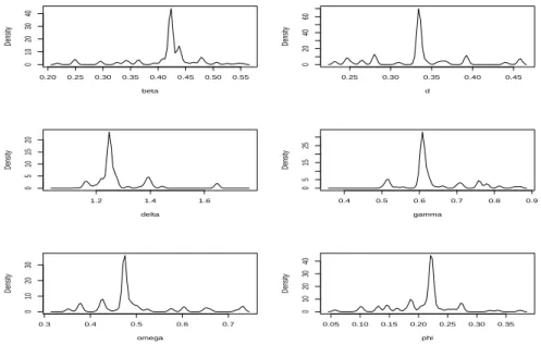
0.20 0.25 0.30 0.35 0.40 0.45 0.50 0.55 0 10 20 30 40 beta Density 0.25 0.30 0.35 0.40 0.45 0 20 40 60 d Density 1.2 1.4 1.6 0 5 10 15 20 delta Density 0.4 0.5 0.6 0.7 0.8 0.9 0 5 15 25 gamma Density 0.3 0.4 0.5 0.6 0.7 0 10 20 30 omega Density 0.05 0.10 0.15 0.20 0.25 0.30 0.35 0 10 20 30 40 phi Density
The density of the marginal posterior samples of the parameters of the FIAPARCH(1,d,1) model are illustrated in Figure (3). Since the graphics show that marginal posterior densities are asymmetric maybe we could use asymmetric priors. It is interesting to notice that these facts are compatible with the results of Bawens and Lubrano (1998) and Dellaportas et al. (2000). These authors point out that the use of asymmetric densities such as gamma or log-normal distributions could generate good results.
0 500 1000 1500 2000 2500 3000 3500 4000 −20 −10 0 10 20 30 returns of IBOVESPA 0 500 1000 1500 2000 2500 3000 3500 4000 0 2 4 6 8 10 12 14 volatility
FIGURE 4: (a) Returns and (b) Posterior mean values of σδ
t - Ibovespa
In Figure (4) we represent graphically the posterior mean of σδ
t, E(σδt|ǫt).
It is possible to see that all periods of great variability of the return of the IBOVESPA were captured by volatility estimated considering δ = 1.2811 and long memory with d = 0.3331.
The good fit of the model is shown in Figure (5) where the residuals standardized are white noise. The absence of heteroskedasticity is noted in the acf for the quadratic residuals standardized.
6
Conclusion
FIAPARCH model is extremely important because it includes several models: long memory models and seven special cases of APARCH models. The performance of the proposed Bayesian approach is good. We notice the
0 10 20 30 40 50 −0.04 −0.03 −0.02 −0.01 0 0.01 0.02 0.03 0.04 0.05 0.06 acf residual 0 10 20 30 40 50 −0.04 −0.03 −0.02 −0.01 0 0.01 0.02 0.03 0.04 0.05 acf residual2
FIGURE 5: ACF of residual, ACF of quadratic residual.
possibility of detecting several particularities such as the long memory and asymmetry.
According to the results obtained by the simulation study and by using IBOVESPA series, the value of the posterior mean estimate of the volatility shows that this analysis has caught extremely well the variability.
In a future research we intend to investigate the effect of using heavy-tailed distributions for the error, for instance, Student or asymmetric t-distributions.
7
References
ANDERSEN, T.; BOLLERSLEV, T. Intraday periodicity and volatility persistence in financial markets. Journal of Empirical Finance, 4, 115-158, 1997.
BAILLIE,R.; BOLLERSLEV,T.; MIKKELSEN,H. Fractionally Integrated Generalised Autoregressive Conditional Heteroscedasticity. Journal of Econo-metrics,, 74, 3-30, 1996.
BAWENS, L.; LUBRANO, M. Bayesian inference on GARCH models using the Gibbs sampler. The Econometrics Journal, Oxford, 1, 23-46, 1998. BOLLERSLEV, T. Generalized Autoregressive Conditional Heteroskedas-ticity. Journal of Econometrics, Lousanne, 31, 307-327, 1986.
BOLLERSLEV,T; MIKKELSEN,H. Modeling and Pricing Long Memory in Stock Market Volatility. Journal of Econometrics, Lousanne, 73, 151-184, 1996.
BOLLERSLEV,T; WOOLDRIDGE,J.M. Quasi-maximum likelihood es-timation and inference in dynamic models with time-varying covariances. Econometric Reviews, 11, 143-172,1992.
CONRAD,C; KARANASOS, M.; ZENG,N. Multivariate Fractionally In-tegrated APARCH Modeling of Stock Market Volatility: A multi-country study,”Working Papers 0472, University of Heidelberg, Department of Eco-nomics, revised Jul 2008.
CRATO,N.;LIMA,P.J.F. Long range dependence in the conditional vari-ance of stock returns. Economics Letters, Amsterdam, 45,281-285, 1994.
DARK, J. A new long memory volatility model with time varying skew-ness and kurtosis. Working Paper, Department of Econometrics and Busi-ness Statistics, Monash University, Australia, 04, 2004.
DAVIDSON, R. Moment and Memory Properties of Linear Conditional Heteroscedasticity Models and a New Model. Journal of Business and Eco-nomic Statistics, 22, 16-29, 2004.
DELLAPORTAS, P.; POLITIS, D. N.; VRONTOS, I. D. Full bayesian inference for GARCH and EGARCH models. Journal of Business and Eco-nomic Statistics, Washington, 18, 187-198, 2000.
DING, Z.; ENGLE, R. F.; GRANGER, C. W. J. A long memory property of stock market returns and a new model. Journal of Empirical Finance, Amsterdam, 1, 83-106, 1993.
DING, Z.; ENGLE, R. F.; GRANGER, C. W. J. Modeling volatility persistence of speculative returns: A new approach. Journal of Econometrics, Lousanne, 73, 185-215, 1996.
ENGLE, R. F.;BOLLERSLEV, T. Modeling the persistence of conditional variances. Econometric Reviews, New York, 5, 81-87, 1986.
GELFAND, A. E.; DEY, D. K.; CHANG, H. . Model determination using preditive distributions with implementation via sampling-based methods. In: BERNARDO, J. M. et al. (Ed.). Bayesian Statistics. Oxford: Oxford University Press., 169-193, 1992.
GELMAN, A.; RUBIN, D.B. Inference from iterative simulation using multiple sequences. Statistical Science, 7, 457-511, 1992.
GEWEKE, J. Evaluating the accuracy of sampling based approaches to the calculation of posterior moments. In: BERNARDO, J. M. et al. (Ed.). Bayesian Statistics. Oxford: Oxford University Press., 169-193, 1992.
GRANGER, C. ; DING.Z. Varieties of Long Memory Models.Journal of Econometrics. 73, 61-77, 1996.
ISLER, J. V. Estimating and forecasting the volatility of Brazilian finance series using ARCH models. The Brazilian Review of Econometrics, Rio de Janeiro, 19, 5-56, 1999.
LIU, M. Modeling long memory in stock market volatility. Journal of Econometrics. 99, 139-171, 2000.
LOBATO, I. ; SAVIN,N. Real and Spurious Long-Memory Properties of Stock-Market Data. American Statistical Association. 16, 261-283,1998.
NELSON,D.B. Stationary and persistence in the GARCH(1,1) model, Econometric Theory, Cambridge, 6, p.6, 318-334,1990.
SILVA, W., S. Uma Abordagem Bayesiana do Modelo ARCH com Potˆen-cia Assim´etrica. Tese apresentada ´a Universidade Federal de Lavras, Lavras, 2006.
TAYLOR, S. Modelling Financial Time Series. New York: John Wiley and Sons, 1986.
TSE, Y. The Conditional Heteroscedasticity of the Yen-Dollar Exchange Rate. Journal of Applied Econometrics, 13, 49-55, 1998.
ZAKOIAN, J. M. Threshold heteroskedasticity models. Journal of Eco-nomic Dynamics and Control, 15, 931-955, 1994.