ARTIFICIAL NEURAL NETWORKS –
AN APPLICATION TO STOCK
MARKET VOLATILITY
Jibendu Kumar Mantri. Deptt. Of Comp.Sc & Applications
North Orissa University Baripada, Orissa Phone (M) 09438084141
Dr. P.Gahan
Deptt. Of Business Administration Sambalpur University,
Sambalpur, Orissa. Phone (M) 09437348150
B.B.Nayak DGM,ECIL RSP,Rourkela Phone (M) 9338493934
Abstract
The present study aims at applying different methods i.e GARCH, EGARCH, GJR- GARCH, IGARCH & ANN models for calculating the volatilities of Indian stock markets. Fourteen years of data of BSE Sensex & NSE Nifty are used to calculate the volatilities. The performance of data exhibits that, there is no difference in the volatilities of Sensex, & Nifty estimated under the GARCH, EGARCH, GJR GARCH, IGARCH & ANN models.
Keywords: GARCH, EGARCH, GJR GARCH, IGARCH, ANN, SISO.MIMO. &ANOVA Test
1.1 Introduction:
Artificial Neural Networks (ANNs) is a statistical technique under the non-linear regression model, discriminant model, data reduction model and non-linear dynamic systems [Sarle -1994; Cheng and Tetterington -1994]. They are trainable analytic tools that attempt to mimic information processing patterns in the brain [Krishnaswamy, Gilbert, Paschley-2000]. ANNs do consider the non-parametric aspects like sentiments, emotions etc. for the estimation of volatilities.
Since ANNs do not require assumptions about the normality of population distribution, financial analysts, economists mathematicians and statisticians are increasingly using ANNs for data analysts.
1.2 The Objectives of the chapter:
1. A multilayer perceptron (MLP) neural network model is used to determine & explore the relationship between some variables as independent factors & the return of the indices as a dependent element. 2. The volatility of Sensex and Nifty under ANNs is compared with the volatility obtained under
GARCH, EGARCH, GJRGARCH & IGARCH models. 1.3 Literature survey:
using different parametric models. They are Mala and Reddy [2007]; Raju & Ghosh [2004]; Batra[2004]; Eckner [2006]; Andrade, Chang and Tabak[2003], Choudhury [2000]; Gulen and Mayhew[2000], Padhi [2004] and many others
White [1988] was the fist to be Neural Networks for stock market fore casting. Ripley [1993] claims that although compressions of ANNs to other methods are rare, however, when done carefully, often show that statistical methods can outperform the state-of the art ANNs. His paper includes a comment from Aharnian [1992] on ANNs as financial applications. Sarle [1994] concludes it is unlikely that ANNs will supersede statistical methodology as he believes that applied statistic is highly unlikely to be reduced to an automatic process or expert system.
Many more works have done to forecast stock market volatility using Neural Networks. Such as Karadi [1997], Aikan [1999], Edolmen [1999], Kammana [1999], Trefalis[1999], Garliauskas, A[1999], Abraham [2000], Sfetsos[2002], Keyong [2004], Lipinsk [2005], De Leone [2006], Xiaotan [2007], Al-Qahari [2008] and Bruce [2009], Mitra [2009]. Similarly Chiang [1996], Kuo [1996], thammaro [1999], Romahi [2000], Marcek Network for analysis stock market volatility. But the statistical approaches descriptive statistics, linear regression, framework GARH family are also used to compare the result of data analysis using NXI for stock market volatility by the researches such as Chan [2000], Resto [2000], Hwang[2001], Dunis[2002], Popesic [2003], Sohn[2005], Leone [2006].
1.4. Data & Methodology:
1.4.1 The Sample
The stock market indices are fairly representative of the various industry sectors and trading activity mostly revolves around the stocks comprising indices. Therefore, the sample of the study consists of the two most important stock indices of India viz. the BSE SENSEX INDEX (Sensex -30) and the NSE NIFTY (Nifty – 50) .Here we analyzed the data from January 1995 to December 2008
1.4.2Research Methodology
I. Volatility Estimation By Using GARCH Group of Models
The basic version of the least squares model assumes that the expected value of error terms, when squared, is the same at any given point of time. This assumption is called homoskedasticity, and it is this assumption which is the focus of GARCH models. Data in which the variances of the error terms are not equal, or in which the error terms may reasonably be expected to be larger for some points of time or smaller at some points, are said to suffer from heteroskedasticity. In the presence of heteroskedasticity, the ordinary least squares (OLS) method of regression solution calculates standard errors and confidence intervals which will be giving a false sense of precision. In stead of considering this as a problem to be corrected, GARCH models to be corrected, GARCH models developed by Engle (1982) and Bollerslev (1986) respectively treat heteroskedasticity as a variance to be modeled.
In financial applications, the return on an asset or portfolio acts as the dependent variable and the variance of the return represents the risk level of those returns. The heteroscedasticity is an issue of time series financial data. The financial data suggests that some time periods are riskier than others. That is, the expected value of the magnitude of error terms at some time period is greater than the others. These risky times are not scattered randomly across monthly, quarter or annual data. There is a degree of auto correlation in the riskiness of financial returns. The amplitude of the returns varies over time is described as volatility clustering GARCH models are designed to deal with just this set of issue. The goal of such models is to provide a volatility measure like a standard deviation – that can be used in financial decisions concerning risk analysis, portfolio selection and derivative pricing.
I.a. GARCH Model
ARCH model has the limitation with respect to the violation of non-negativity constraints. To overcome these limitation GARCH model was developed independently by T. Bollerslev in 1986 and S. J. Taylor in 1987. They suggested that the conditional variance be specified through GARCH (q, p) model as
2 2
0
1 1
ˆ
ˆ ˆ
ˆ ˆ
q p
t i t q j t j
i j
u
……….. eqn..20
0;
i
0
, for i= 1,2,……….q0,
j
for j- 1,2,……….….pto ensure a positive conditional variance.
Thus the volatility is expressed as a function of
0, a constant,u
ˆ
2t i news about volatility from the previous period ‘t-1’ (the ARCH term) and
ˆ
2t j , the previous periods forecast variance (The GARCH term). The conditional variance can be expressed as2 0
1 1
1 t
under GARCH(1,1).
Thus, for the conditional variance to exist, the GARCH model requires a restriction on
1
1
1
.Banarjee and Sarkar (2006) claim that the Indian stock market exhibits volatility clustering and hence, GARCH type of models can better predict the market volatility.
In the present study, GARCH (1, 1), GARCH (2, 2) and GARCH (3, 3) are used to estimate the volatility of BSE SENSEX and NSE NIFTY, 50 stocks.
I.b. EGARCH (Exponential GARCH) model
GARCH model is based on the assumption of symmetric treatment of positive and negative shocks. However, it has been observed and reported that volatility in a rising market is less than the volatility in a falling market. This asymmetry is attributed to leverage effect, whereby a fall in the value of a firm’s stock causes the debt to equity ratio to rise which in turn leads the share holders who undertake the unsystematic risk of the company to perceive their future cash flow stream as being more risky. This feature was first documented by Black (1976) and Christie (1982). Empirical evidence can also be found in Nelso (1991), Gallant et_al (1992), Campbell and Kyle (1993) and Engle and Ng (1993); Nelso (1991) also proposed an exponential GARCH (E GARCH) framework to model volatility under the conditions of asymmetric reaction of the investors / leverage effect.The present study and EGARCH (3, 3) in order to estimate the volatility of Indian stock market under the condition of asymmetric behaviour of the investor in a rising and falling markets.
The EGARCH (p, q, r) model is specified below:
2 2 1 1
1
1 1
ˆ
ˆ
log(
)
log(
)
t t...3
t
t t
u
u
t
w
The log of the conditional variance implies the leverage effect is exponential. The last term of the above equation captures the asymmetric impact.
is the GARCH term that measures the impact of last period’s forecast variance. A positive indicates volatility clustering implying that positive stock price changes are associate with further positive changes and vice versa.
is the ARCH term that measure that effect of news about volatility from the previous period on current period volatility. measures the leverage effect. Ideally is expected to be negative implying that bad news has a bigger impact on volatility than goods new of the same magnitude. A persisted volatility shock raises the unit price volatility.
I.c. I. GARCH (Integrated GARCH)
One of the restrictions in GARCH model is that the value of and equals unity, there would be an unit root variance and is termed as Integrated GARCH. I GARCH is used to estimate volatility if the current shocks persist indefinitely in conditioning future variances [Engle and Bollerslev, 1986; Nelson, 1990].
I.d. GJR GARCH Model (Glosten, Jagannathan and Runkle GARCH)
2 2 2 2 0
1 1 1
ˆ
ˆ
ˆ
ˆ
q q p
t i t i i t i t i j t j
i i j
u
u
I
Where,
I
t1 = 1 ifu
t1
0
0
other wiseFor the leverage effect, >o. The condition for non negativity will be >0, 1 0, 0, is the asymmetry term
.
I.e MLP Model
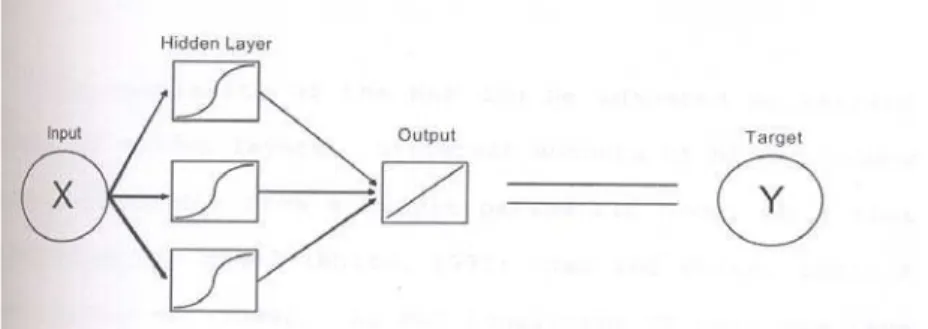
One of the most useful and successful applications of neural networks to data analysis is the multilayer perceptron model (MLP). Multilayer perceptron models are non-linear neural network models that can be used to approximate almost any function with a high degree of accuracy (white 1992). AN MLP contains a hidden layer of neurons that uses non-linear activation functions, such as a logistic function. Figure 1 offers a representation of an MLP with one hidden layer and a single input and output. The MLP in figure 1 represents a simple non-linear regression.
Figure 1: Multi-layer Perceptron with a Single input and Output
The number of inputs and outputs in the MLP, as well as the number, can be manipulated to analyze different types of data. Figure2 presents a multilayer perceptron with multiple inputs and outputs. This MLP represents multivariate multiple nonlinear regression.
Figure 2: Multi-layer Perceptron with Multiple inputs and outputs.
1.5 Analysis of Results
Table-1-Daily Volatility of Sensex and Nifty under MLP Technique of ANNs Model (In percent)
Sensex Volatility Nifty Volatility
Year SISO MISO SISO MISO
1995 1.03515 1.12268 1.1349 1.10025
1996 1.01753 1.20147 1.14972 1.2309
1997 1.07989 1.31996 1.05076 1.30627
1998 1.41298 1.40189 1.22769 1.37131
1999 1.33452 1.43588 1.15444 1.42019
2000 1.74905 1.84146 1.60518 1.46947
2001 1.08309 1.31508 1.01619 1.28586
2002 0.72298 0.84885 0.65202 0.80301
2003 0.76205 0.98956 0.79634 0.96407
2004 0.75012 1.1907 0.90385 1.19244
2005 0.64083 0.95566 0.61568 0.96189
2006 0.85601 1.25608 1.51564 1.29434
2007 1.09288 1.47939 1.4174 1.42525
2008 1.98115 2.51065 1.75171 2.34098
NB: SISO: Single Input Single Output MISO: Multiple Inputs Single Output.
The daily volatilities obtained in each year over 1995-2008 under single input as low index level and single out as high index lever are less than what has been obtained under multiple inputs as opening, high and low index levels and single output as the closing index level through the MLP of ANNs in case of Sensex. Volatilities during 1995-2000 are showing an increasing trend consistently in single layer as well as multilayer training method of MLP in ANNs in case of Sensex. In case of Single layer trainable system, volatility has increased to 1.749% in 2000 from a low volatility of 1.035% in 1995. In case of multilayer trainable system, volatility has risen to 1.841% in 2000 from a low of 1.123% in 1995. Volatility has started declining from the year 2001 to 2006 consistently in both the trainable systems (single and multiple). Hence, the period 2001 to 2006 can be considered as a period of relative calm which may be the result of financial derivatives like options and futures on indices. From a high value of 1.74% in 2000, volatility declined to 0.85% under single layer in 2006 and from a high value of 1-84% in 2000, it has declined to 0.956% in 2005 and 1.256% in 2006. After 2006, the volatility again has showed a rising trend. The rising trend in volatility is attributed to the global financial crisis and its impact on Indian stock market.
Similar results are obtained in case of Nifty under both single layer and multi layer, trainable techniques of MLP of ANNs model. The volatility in Nifty has increased to 1.60% in 2000 from a low of 1.35% in 1995 in case of single input as low index level and single out as high index level of MLP. The period of relative calm as observed from 2001 to 2005 where the volatility has been drastically reduced to 0.615% in 2005 from a high of 1.605% in 2000. The reason is due to the aggressive use of derivatives in NSE in comparison to the BSE. But after 2005, again there is the rise of volatility and it has shot up to 1.75% in 2008 from a low of 0.615% which is almost 300% rise in volatility within three years. This is due to the world-wide financial crisis. Under multiple inputs and single output trainable technique of MLP of ANNs, similar results of rising and falling trends are observed. In this case, volatility in Nifty has risen to 1.47% in 2000 from a low of 1.1% in 1995. From 2001-2005, volatility has showed a declining trend where volatility has been reduced to 0.96% in 2005 from a high of 1.47% in 2000.
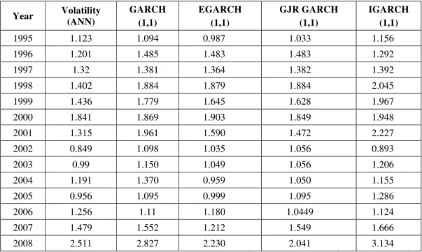
Table 2 presents the volatility of ANN model along with GARH, EGARCH, GJR GARCH and IGARCH models for Sensex for the period January 1995 - December 2008.
Table 2-Year wise Daily volatility of Sensex under ANN models and GARCH Family of Models (in percent)
Year Volatility
(ANN)
GARCH (1,1)
EGARCH (1,1)
GJR GARCH (1,1)
IGARCH (1,1)
1995 1.123 1.094 0.987 1.033 1.156
1996 1.201 1.485 1.483 1.483 1.292
1997 1.32 1.381 1.364 1.382 1.392
1998 1.402 1.884 1.879 1.884 2.045
1999 1.436 1.779 1.645 1.628 1.967
2000 1.841 1.869 1.903 1.849 1.948
2001 1.315 1.961 1.590 1.472 2.227
2002 0.849 1.098 1.035 1.056 0.893
2003 0.99 1.150 1.049 1.056 1.206
2004 1.191 1.370 0.959 1.050 1.155
2005 0.956 1.095 0.999 1.095 1.286
2006 1.256 1.11 1.180 1.0449 1.124
2007 1.479 1.552 1.212 1.549 1.666
2008 2.511 2.827 2.230 2.041 3.134
The Volatility under ANN model is less than that of the volatility from GARCH model. The GARCH model is symmetric in nature and therefore gives equal weightage to both positive and negative shocks while calculating volatility. For this above reason, volatility under GARCH model may not appropriately find a place in option valuation and portfolio selection models. It is the volatility under ANN model which may be used for option pricing and portfolio selection as it takes care of non-linearity in data by removing outliers and sentiments of the traders.
EGARCH and GJR GARCH models are best known as asymmetric models. These models are based on the fact that negative shocks bring more fluctuation (decline in value) than the positive events (increase in value) in indices or in individual securities. It’s because the investors are more affected sentimentally due to the arrival of bad news to the market than that of the good news. Volatility calculation under ANN models since takes care of both sentimental factors as well as outliers. It is to be considered as a better model than the asymmetric models. Volatility obtained under ANN model is less than that of EGARCH and GJR GARCH models in most of the years as has been seen in Table 2 for Sensex.
Volatility under IGARCH model deals with the persistence of shocks in the market. This model helps the trader to know whether the impact of the present shock on the price of the stock will remain for a short period/ long period/ infinite period. This type of information can’t be obtained from the ANN model. The table 2 shows that the volatility of GARCH, EGARCH, GJR GARCH, IGARCH models is also more than the volatility of ANN model.
Table 3-ANOVA results Sensex volatility under ANN, GARCH, EGARCH, GJRGARCH and IGARCH models
Anova: Single
Factor
SUMMARY
Groups Count Sum Average Variance
Column 1 14 18.87 1.347857 0.173961
Column 2 14 21.655 1.546786 0.238717 Column 3 14 19.515 1.393929 0.164705 Column 4 14 19.6229 1.401636 0.126636
Column 5 14 22.491 1.6065 0.362878
ANOVA Source of Variation SS df MS F P-value F crit Between Groups 0.690756 4 0.172689 0.809305 0.523765 2.51304
Within Groups 13.86965 65 0.213379
Total 14.5604 69
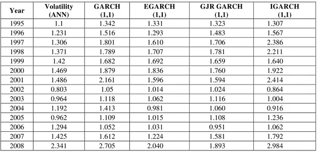
Table -4 shows the volatility of Nifty under ANN, GARCH, EGARCH, GJR GARCH and IGARCH models for the periods January 1995- December 2008.
Table 4-Year wise Daily volatility of Nifty under ANN models and GARCH Family of Models (in percent)
Year Volatility
(ANN)
GARCH (1,1)
EGARCH (1,1)
GJR GARCH (1,1)
IGARCH (1,1)
1995 1.1 1.342 1.331 1.323 1.307
1996 1.231 1.516 1.293 1.483 1.567
1997 1.306 1.801 1.610 1.706 2.386
1998 1.371 1.789 1.707 1.781 2.211
1999 1.42 1.682 1.692 1.659 1.640
2000 1.469 1.879 1.836 1.760 1.922
2001 1.486 2.161 1.596 1.594 2.414
2002 0.803 1.05 1.014 1.024 0.864
2003 0.964 1.118 1.062 1.116 1.004
2004 1.192 1.413 0.981 1.060 0.916
2005 0.962 1.109 1.015 1.108 1.236
2006 1.294 1.052 1.031 0.951 1.062
2007 1.425 1.612 1.224 1.581 1.792
2008 2.341 2.705 2.040 1.893 2.984
It is seen from the above table that the volatility of Nifty under ANN model is also less than the volatility obtained from GARCH, EGARCH, GJR GARCH AND IGARCH models. Similar interpretations can be made here like that of Sensex while comparing ANN model with that of GARCH, EGARCH, GJR GARCH and IGARCH model of volatility.
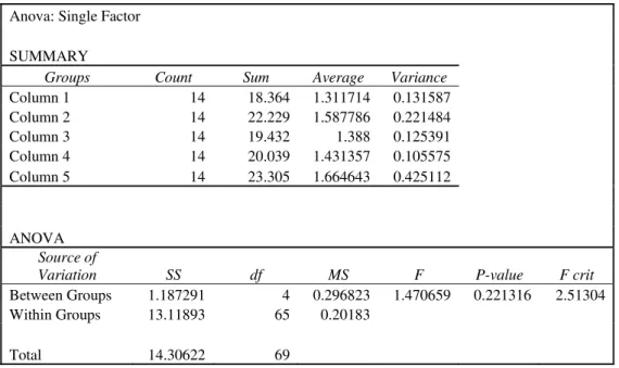
Table-5---ANOVA results Nifty volatility under ANN, GARCH, EGARCH GJRGARH and IGARCH models
Anova: Single Factor
SUMMARY
Groups Count Sum Average Variance
Column 1 14 18.364 1.311714 0.131587
Column 2 14 22.229 1.587786 0.221484
Column 3 14 19.432 1.388 0.125391
Column 4 14 20.039 1.431357 0.105575
Column 5 14 23.305 1.664643 0.425112
ANOVA Source of
Variation SS df MS F P-value F crit
Between Groups 1.187291 4 0.296823 1.470659 0.221316 2.51304
Within Groups 13.11893 65 0.20183
Total 14.30622 69
It is observed from the above table that the F-calculated value is less than the F-critical value at 22.13% significance level. From this, it is concluded that there is no difference in the volatilities estimated under the different models under consideration here. So, the traders, financial analyst and others should remain indifferent in using any method to estimate volatility Fig3& Fig4 presents a graphical view of the volatilities under all the models used here.
Fig 3-Year wise Volatility of Sensex- MISO, GARCH(1, 1), EGARCH (1, 1), GJRGARCH (1, 1), IGARCH(1, 1)
BSE SENSEX-ANN,GARCH,EGARCH,GJR,IGARCH
0 5 10 15
199 5
19961997199 8
1999200 0
20012002200 3
2004200 5
20062007200 8
Year
V
o
la
tili
ty IGARCH
GJR
EGARCH
GARCH
ANN
Fig 4- Year wise Volatility of Nifty - MISO, GARCH (1, 1), EGARCH (1, 1), GJRGARCH (1, 1), IGARCH(1, 1)
NSENIFTY-ANN,GARCH,EGARCH,GJR,IGARCH
0 5 10 15
1995199619971998199920002001 2002200320042005200620072008
Year
V
o
la
ti
lit
y
IGARCH
GJR
EGARCH
GARCH
ANN
Conclusion:
ANN model is less than that of the GARCH, EGARCH, GJR GARCH and IGARCH models, ANOVA test is being conducted to conclude that there is no difference in the volatility estimated by the different models. Hence, the traders, financial analysts and economists may remain indifferent while choosing the model and the estimation of volatility
References:
[1] Abraham, A., B. Nath and P. K. Mahanti. (2001) "Hybrid Intelligent Systems for Stock Market Analysis," Computational Science, Springer-Verlag Germany, Vassil N. Alexandrov et. al. (Eds.), ISBN 3-540-42233-1, San Francisco, USA, 337-345
[2] Aharonian, G., (1992) Comments on comp.ai.neural-nets, Items 2311 and 2386 [Internet Newsgroup].
[3] Aiken, M. and M. Bsat. (1999) “Forecasting Market Trends with Neural Networks.” Information Systems Management 16 (4)”, 42-48. [4] Al-Qaheri H., Hassanien A. E., Abraham A( 2008), “Discovering stock price prediction rules using rough sets, Neural Network
World“, Vol. 18, 181-198
[5] Black, F. (1976), ‘Studies in stock Price volatility changes,’ Proceedings of the 1976 Business Meeting of the Business and Economic Statistics section, American Statistical Association, 177-181
[6] Banerjee, A. and Sarkar, S. (2006), ‘Modeling daily volatility of the Indian stock market using intra-day data,’ working paper series No. 588/March, Indian Institute of Management Calcutta
[7] Bruce Vanstone &Gavin Finnie,- (2009) “An empirical methodology for developing stock market trading systems using artificial neural networks, An International Journal of Expert Systems with Applications”, Volume 36 , Issue 3 , 6668-6680
[8] Chan, M-C, C-C Wong, and C-C Lam. (2000) “Financial Time Series Forecasting by Neural Network Using Conjugate Gradient Learning Algorithm and Multiple Linear Regression Weight Initialization,” Department of Computing, The Hong Kong Polytechnic University, Kowloon, Hong Kong
[9] Cheng, B. and D.M. Titterington, 1994, “Neural Networks: A Review from a Statistical Perspective,” Statistical Sciences, 9(1), 2-54. [10] Chiang, W.-C., T. L. Urban and G. W. Baldridge. (1996) “A Neural Network Approach to Mutual Fund Net Asset Value Forecasting.”
Omega, Int. J. Mgmt Sci. 24 (2), 205-215.
[11] Christie, A.A. (1982), ‘The Stochastic Behaviour of common stock Variances: value, leverage and Interest rate Effects,’ Journal of Financial Economics, 10, 407-432
[12] De Leone R., Marchitto E., Quaranta A. G. ( 2006), “Autoregression and artificial neural networks for financial market forecast, Neural Network World,“ Vol. 16, 109-128
[13] Deboeck G.J. ,Ultsch A. (2000), “Picking stocks with emergent self-organizing value maps, Neural Network World“ , Vol. 10,203-216 [14] Dunis C.L. Laws J. Chauvin S. (2000), “FX volatility forecasts: a fusion-optimisation approach, Neural Network World“, Vol. 10,
,187-202
[15] Edelman, D., P. Davy and Y. L. Chung. (1999) “Using Neural Network Prediction to achieve excess returns in the Australian All-Ordinaries Index”. In: Queensland Financial Conference, Sept 30th & Oct 1st, Queensland University of Technology
[16] Engle, R.F. (1982), ‘Autoregressive conditional heteroskedasticity with estimates of the variance of UK inflation,’ Econometrica, 41, 135-155.
[17] Engle R and Bollerslev.T (1986) Modeling the persistence of conditional variances. Econo- metric Reviews, 5:1 50, 1986 [18] Engle, R.F. and Ng, V.K (1993), ‘Measuring and Testing the impact of news on volatility,’ Journal of Finance, 48, 1749-1801 [19] Gallant, A.R., Rossi, P.E. and Touchen, G. (1992), ‘Stock prices and volume’, Review of Financial Studies, 5, 199-242.
[20] Garliauskas, A. (1999) “Neural Network Chaos and Computational Algorithms of Forecast in Finance.” Proceedings of the IEEE SMC Conference on Systems, Man, and Cybernetics 2, 638-643. 12-15 October
[21] Ghaziri H ,Elfakhani S. Assi J. , (2000), “Neural networks approach to pricing options, Neural Network World, Vol. 10,271-277 [22] Gilbert, E.W., C.R. Krishnaswamy, and M.M. Pashley, 2000, “Neural Network Applications in Finance: A Practical Introduction,”. [23] Gleitman, H., (1991), Psychology, W.W. Norton and Company, New York.
[24] Hwarng, H. B. (2001) “Insights into Neural-Network Forecasting of Time Series Corresponding to ARMA (p, q) Structures.” International Journal of Management Science, Omega, 29, 273-289.
[25] Karali, O. Edberg, W. Higgins, J. Motorola Inc., Schaumburg, (1997)” Modelling volatility derivatives using neural networks, Computational intelligence for Financial Engineering (CIFEr), 1997, Proceedings of the IEEE/ IAFE 1997, 280-286.
[26] Kollias, C. and A. Refenes, (1996), “Modeling the Effects of Defense Spending Reductions on Investment Using Neural Networks in the Case of Greece,” Center of Planning and Economic Research, Athens.
[27] Kuo, R. J., L. C. Lee and C. F. Lee. (1996) “Integration of Artificial Neutal Networks and Fuzzy Delphi for Stock Market Forecasting.” IEEE, June, 1073-1078.
[28] Kyoung-Jae Kim ,Boo Lee (2004), “Stock market prediction using artificial neural networks with optimal feature transformation: Neural Computing and Applications“ 255 - 260
[29] Lipinski P. (2005), “Clustering of large number of stock market trading rules, Neural Network World“, Vol. 15, 351-357
[30] Maasoumi, E., A. Khotanzad, and A. Abaye, (1994), “Artificial Neural Networks for Some Macroeconomic Series: A First Report,” Econometric Reviews, 13(1), 105-22.
[31] Majhi R., Panda G., Majhi B., Sahoo G., (2006), “Efficient prediction of stock market indices using artificial adaptive bacterial foraging optimization (ABFO) and BFO based techniques” Expert Systems with Applications: An international journal, pp.10097-10104
[32] Michalak K., Lipinski P.( 2005), “Prediction of high increases in stock prices using neural networks, Neural Network World“, Vol. 15, 359-366
[33] Mitra Subrata Kumar (2009), “Optimal Combination of Trading Ruls Using Neural Networks” International Business Research, Vol 2, No.1.pp. 86-99.
[34] Nelson, D., (1990) 'Conditional heteroskedasticity in asset retums: a new approach' Econometrica. 59 , 347-70 [35] Nelson, D.B. (1991), ‘Conditional heteroskedasticity in asset returns : a new approach,’ Econometrica, 53, 347-370
[36] Popescu Th. D. (2003), “Change Detection in Nonstationary Time Series in Linear Regression Framework, Neural Network World“, Vol. 13, 133-150
[37] Resto M. TRN; (2000), “Picking up the challenge of non linearity testing by means of topology representing networks, Neural Network World“, Vol. 10,173-186
[39] Roger, L CG, Satchell, SE (1991) “ Estimating variance from High, Opening & Closing Price annals of applied probability,1(4),504-512
[40] Romahi, Y. and Q. Shen. (2000) “Dynamic Financial Forecasting with Automatically Induced Fuzzy Associations.” IEEE, 493-498 [41] Sarle, W.S., 1994, “Neural Networks and Statistical Models,” Proceedings of the Nineteenth Annual SAS Users Group International
Conference, Cary, NC: SAS Institute, April, 1538-1550.
[42] Sfetsos A. (2002), “The application of neural logic networks in time series forecasting, Neural Network World“, Vol. 12, 181-199 [43] Sohn S. Y, Shin H. W. ( 2005), “EWMA combination of both GARCH and neural networks for the prediction of exchange rate, Neural
Network World“, Vol. 15, 375-380
[44] Thammaro, A. (1999) "Neuro-fuzzy Model for Stock Market Prediction," in Dagli, C. H., A. L. Buczak, J. Ghosh, M. J. Embrechts, and O. Ersoy (Eds.) Smart Engineering System Design: neural networks, fuzzy logic, evolutionary programming, data mining, and complex systems. Proceedings of the Artificial Neural Networks in Engineering Conference (ANNIE '99). New York: ASME Press, 587-591
[45] Trafalis, T. B. (1999) "Artificial Neural Networks Applied to Financial Forecasting,” in Dagli, C. H., A. L. Buczak, J. Ghosh, M. J. Embrechts, and O. Ersoy (Eds.) Smart Engineering Systems: Neural Networks, Fuzzy Logic, Data Mining, and Evolutionary Programming, Proceedings of the Artificial Neural Networks in Engineering Conference (ANNIE'99). New York: ASME Press, 1049-1054.
[46] White, H. (1988) "Economic Prediction Using Neural Networks: The Case of IBM Daily Stock Returns" in Proceedings of the Second Annual IEEE Conference on Neural Networks, II: 451-458
[47] White, H., 1992, Artificial Neural Networks: Approximation and Learning Theory, With A. R. Gallant, Cambridge and Oxford: Blackwell.