Optimal Scheduling of Joint Wind-Thermal Systems

(1)

Optimal Scheduling of Joint Wind-Thermal Systems

R. Laia1,2_{, H.M.I. Pousinho}1_{, R. Melício}1,2_{, V.M.F. Mendes}2,3,4

1_{IDMEC, Instituto Superior Técnico, Universidade de Lisboa, Lisbon, Portugal} 2_{Departamento de Física, Escola de Ciências e Tecnologia, Universidade de Évora.}

3_{Instituto Superior de Engenharia de Lisboa, Lisbon, Portugal,}_{ruimelicio@gmail.pt} 4_{C‐MAST Center for Mechanical and Aerospace Sciences and Technology}

Abstract. This paper is about the joint operation of wind power with thermal power for bidding in day-ahead electricity market. Start-up and variable costs of operation, start-up/shut-down ramp rate limits, and ramp-up limit are modeled for the thermal units. Uncertainty not only due to the electricity market price, but also due to wind power is handled in the context of stochastic mix integer linear programming. The influence of the ratio between the wind power and the thermal power installed capacities on the expected profit is investigated. Comparison between joint and disjoint operations is discussed as a case study. Keywords: Stochastic; Mixed integer linear programming; Wind-thermal.

1 Introduction

Renewable energy sources play an important role in the need for clean energy in a sustainable society [1]. Renewable energy can partly replace fossil fuels, avowing anthropogenic gas emissions. Energy conversion from renewable energy has been supported by policies, providing incentive or subsidy for exploitation [2]. These polices have pushed the integration of renewable energy forward, but by an extra-market approach. The approach involves, for instances, legislative directives, feed-in tariffs, favorable penalty pricing and grid right of entry, and survives at reserved integration level. But as integration of renewable energy increases the approach is expected to be untenable [3]. Sooner or later, a wind power producer (WPP) has to face competition in a day-ahead electricity market. For instances, in Portugal, a WPP is paid by a feed-in tariff under the condition of a limited amount of time or of energy delivered. Otherwise, the route is the day-ahead market or by bilateral contracting [4].

Conversion of wind energy into electric energy to trade in the day-ahead electricity market has to face uncertainty, particularly, on the: availability of wind energy, energy price and imbalance penalty. These uncertainties have to be addressed to avoid dropping profit [5-7]. A stochastic programming addresses uncertainty by the use of modeling via scenarios, and is a suitable approach to aid a Wind-Thermal Power Producer (WTPP) in developing a joint bid strategy in a day-ahead market [8-12]. The problem formulation is approached in a way of approximating all expressions regarding the objective function and the constraints to describe the problem by a mixed integer linear program (MILP) one. The approximation is intended to use excellent commercial available for MILP. The uncertainties are treated by uncertain measures and multiple scenarios built by wind power forecast [13-15] and market-clearing electricity price forecast [16-18] applications.

(2)

A case study with data from the Iberian Electricity Market is used to illustrate the effectiveness of the proposed approach. The approach proves both to be accurate and computationally acceptable.

2 Problem Formulation

2.1 Market Balancing

System imbalance is defined as a non-null difference on the trading, i.e., between physical delivered of energy and the value of energy on contract at the closing of the market. If there is an excess of delivered energy in the power system, the system imbalance is positive; otherwise, the system imbalance is negative. The system operator seeks to minimize the absolute value of the system imbalance in a power system, using a mechanism based on prices penalization for producer imbalance, i.e., the difference of the physical delivery of energy from the one accepted due to the bid of the producer. If the system imbalance is negative, the system operator keeps the price for the physical delivery of bided energy for the producers with positive imbalance and pays a premium price for the energy produced above bid. The revenue

t

R of the producer in hour t is given by [19]:

t offer t D t t P I R   (1) In (1), offer t

P is the power traded by the producer in the day-ahead market and It is the imbalance income resulting from the balancing process, offer

t D t P

 is the revenue that the producer collects from trading energy if there is no uncertainties. The deviation of the producer in hour t is given by:

offer t act t tP P  (2) In (2), act t

P is the physical delivery of energy in hour t. Two ratio prices for positive and negative imbalances are, respectively, given by:

1 ,      t D t t t r r   _; 1 ,      t D t t t r r   (3)

In (3), t is the price paid by the market to the producer for a positive imbalance,



t

 is the price to be charged to the producer for a negative imbalance. The imbalance in (1) using (3) is given by:

0 ,      t t t D t t r I  ;  tt, t 0 D t t r I  (4)

A producer that needs to correct its energy imbalance in the balancing market incurs on an opportunity cost, because energy is traded at a more profitable price in the day-ahead market.

(3)

The imbalance in (2) will cause an opportunity cost given by: 0 , ) 1 (       t t t D t t r C  ; C_tD_t (r_t1)_t,_t0 (5)

The uncertainties are considered by a set of scenarios  for wind power, energy price and ratio prices for system imbalance. Each scenario  will be weighted with a probability of occurrence  .

2.2 Thermal Production

The operating cost Fitin scenario for a thermal unit i in hour tis given by [20]: t i z C b d u A F_i_t _i _i_t _i_t _i_t _i _i_t ,  ,  ₍₆₎ In (6), the operating cost is composed by four terms, namely: Ai is a fixed operating

cost; dit is a variable cost, i.e., is a part of the cost incurred by the amount of fossil

fuel consumed above the minimum power; bit is the unit start-up cost; Ci is the

unit shut-down cost. The typical non-differentiable and nonconvex functions used to quantify the variable costs of a thermal unit is replaced by a piecewise linear approximation in order to take the advantage of using MILP [5]. The piecewise linear approximations for the variable cost dit is formulated by the statements given by:

t i F d L l l i l i t i 



    , , 1 t    (7) t i u p p L l l t i t i i  



    , , 1 i min t     (8) t i t p Ti  i ) _i_t _i_t  ,  ,  ( 1 min 1_ _1  ₍₉₎ t i u p Ti i _i_t t i (  )  ,  ,  min 1 1 _ _ _ (10) 1 ,.., 2 , , , ) (T Til1tl it l_i_t  i t l L l i    ₍₁₁₎ 1 ,.., 2 , , , ) (  1 1        T_il T_il tl_i_t i t l L l t i  _ _ (12) t i t T pi Lit Lit L t i       (  )  , , 0  max  1 1  ₍₁₃₎

In (7), the variable cost is computed as the sum of the product of the slope of each segment l

i

F by the segment power l t i 

(4)

given by the minimum power production plus the sum of the segment powers associated with each segment. The binary variable uit ensures that the power

production is equal to 0 if unit i is offline. In (9), if the binary variable l t i

t_ has a null value, then the segment power 1

t i 

 can be less than the segment 1 maximum power; otherwise and in conjunction with (10), if the unit is on, then 1

t i 

 is equal to the segment 1 maximum power. In (11), from the second segment to the second last one, if the binary variable l

t i

t_ has a null value, then the segment power l t i 

 can be less than the segment l maximum power; otherwise and in conjunction with (12), if the unit is on, then l

t i 

 is equal to the segment l maximum power. In (13), if the binary variable L 1

t i

t_ has a null value, then the segment power L must be zero; otherwise is bounded by the last segment maximum power.

The exponential nature of a start-up cost of thermal units is modelled by an approximation of a non-decreasing stepwise function with a step [5] given by:

t i u u K b r r t i t i i t i _           



  , , 1       (14) t i b_i_t0 ,  ,  ₍₁₅₎

In (14), if in scenario  unit i in hour t is online and has been offline in  preceding hours, the expression in parentheses is equal to one, implying that a start-up happen in hour t and the respective cost K_i is incurred.

The box constraints for the power production in scenario  of unit i in hour t are given by: t i p p u pi it  it  it  ,  ,  max min     ₍₁₆₎ t i z SD z u p pmax_i_t  _imax( __i_t __i_t_₁) __i_t_₁, , ₍₁₇₎ t i y SU u RU p p_max_i_t  max__i_t_₁ __i_t_₁ __i_t, , ₍₁₈₎ t i z SD u RD p p__i_t_₁ __i_t __i_t __i_t, , ₍₁₉₎

In (16), the power limits of the units are set. In (17) and (18), the upper bound of max

t i

p is set, which is the maximum available power in scenario  for a thermal unit i

in hour t. This variable considers the: actual power of a unit, start-up/shut-down ramp rate limits, and ramp-up limit. In (18)–(19), the relation between the start-up and shut-down variables of the unit are given, using binary variables and their weights. In (19), the ramp-down and shut-down ramp rate limits are considered.

(5)

The minimum down time constraint is imposed by a linear formulation given by: i u i J t t i   



 , 0 1   (20) 1 ... 1 , , ) 1 ( 1         



   i i t i i DT k k t t i DT z i k J T DT u i    (21) T DT T k i z u i T k t t i t i ) 0 , , 2... 1 (         



    (22) )} 1 )( ( , min{ _i _i₀ _i₀ i T DT s u J      ₍₂₃₎

In (21), the minimum down time is satisfied for all the possible sets of consecutive hours of size DTi, and in (22) is satisfied for the last DTi 1 hours.

The minimum up time constraint is imposed by linear formulation given by: i u i N t t i    



 , 0 ) 1 ( 1   (24) 1 ... 1 , , 1        



   i i t i i UT k k t t i UTy i k N T UT u i    (25) T UT T k i z u _i T k t t i t i ) 0 , , 2... (        



    (26) } ) ( , min{ i i0 i0 i T UT U u N     ₍₂₇₎

In (24), the minimum up time is satisfied for all the possible sets of consecutive hours of size UTi. In (25), the minimum up time will be satisfied for the last UTi1. The

relations between the binary variables to identify start-up and shutdown are given by:

t i u u z y__i_t __i_t __i_t __i_t_₁, , (28) t i z y__i_t __i_t 1 ,  ,  (29)

The total power produced by the thermal units is given by: t p p I i t i g t 



   , 1    (30)

In (30), I is the set of indexes for the thermal units, g t

p_ is the total thermal power in scenario  in hour t.

(6)

The total operating costs T t

F of the thermal power system is given by:

t F F I i t i T t



   , 1    (31)

In (31), the operating cost Fit in scenario  for unit i in hour is given by (5). 2.3 Objective Function

The power in the bid submitted by the WTPP is the sum of the power from the thermal power system with the power from the wind power system and is given by:

D t th t offer t p p p_  _  _ ; p p p d t t g t act t   ,      ₍₃₂₎ In (32), g t

p_ is the actual power of the thermal power system and d t

p_ is the actual power of the wind power system produced for scenario . The expected revenue of the WTPP over the time horizon NT is given by the solution of the following mathematical programing problem with the objective function given by:



           __      _ _ _ _ N N t T t t t D t t t D t offer t D t T F r r P 1 1                (33) Subject to: t p poffer_t  M_t    , 0    ₍₃₄₎



pact_t poffer_t



t t        , ₍₃₅₎ t t t t        __,    ₍₃₆₎ t d P_t _t t       _, 0    ₍₃₇₎ t p p p E I i t i M t



    , max 1 max _   (38) In (34), M t

p_ is the maximum available power (38), limited by the sum of the installed capacity in the wind power system, Emax

p , with the maximum thermal production. Some day-ahead markets require that the bidding to be submitted is given by:

t p

poffer_t  offer_t )( D_t D_t)0  , ', 

( _ __' _ __'  

(39)

In (39), if the day-ahead market prices are equal for two scenarios  and ' then the power bid difference between the two scenarios is indifferent. Otherwise, the power bids have to be non-decreasing with the price. Non decreasing energy bids are assumed. Hence, when wind power and thermal power bids are disjoint submitted implies that each bid has to be a decreasing one. While, only one joint non-decreasing bid is submitted in the joint schedule.

(7)

3 Case Study

The simulations are carried out in Gams using the Cplex solver for MILP. The effectiveness of the stochastic MILP approach is illustrated by a case study using a set of data from the Iberian electricity market, comprising 10 days of June 2014 [21]. The scenarios for the energy prices and the energy availability for the wind power system are respectively in the left and right sides of Fig. 1.

Fig 1. June 2014 (ten days); left: Iberian market price, right: wind energy. The producer owns a wind power system with an installed capacity of 360 MW and a thermal power system with 8 units and a total installed capacity of 1440 MW. The variable costs of the thermal units are modelled by three segments in the piecewise linear approximation. Firstly, the simulations are carried out with the previous values of the installed capacities in order to find the expected profit and the expected imbalance cost without joint schedule, i.e., for the wind power and for the thermal power systems standing alone, and with joint schedule. The expected profit and the expected imbalance cost without and with joint schedule are shown in Table 1.

Table 1. Results without and with joint schedule

Case Study Profit (€) Imbalance Cost (€)

Wind system 119200 -17826

Thermal system 516848 229398

Disjoint wind and thermal systems 636047 …

Wind-thermal system 642326 3643

Gain (%) 0.99 …

In Table 1, the expected profit of the joint schedule is 0.99% higher than the disjoint one and the processing is not a burden in computational resources in comparison with the disjoint one: the CPU time given by Gams is about the same for both schedules, since the wind power system schedule CPU time is irrelevant when compared with the thermal power system one in the disjoint schedule. Information for hour 15 regarding the sum of the wind power with the thermal power bid without and with joint schedule is shown in Fig. 2.

(8)

Fig 2. Bid of energy for hour 15; left: disjoint, right: joint.

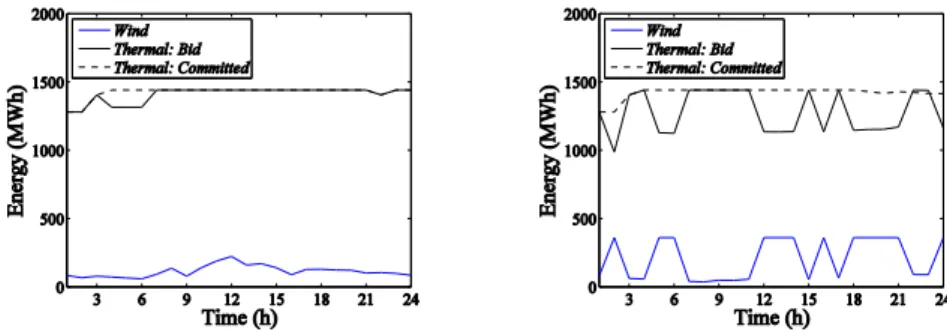
In Fig. 2, note that wind and thermal power do not have to be non-decreasing per se. The energy bids in scenario 3 for the disjoint and joint schedule are respectively in the left and right figures of Fig. 3.

Fig 3. Bid of energy and committed in scenario 3; left: disjoint, right: joint.

The wind parcel of the energy bid is higher for the joint schedule and the thermal bid behavior tends to be the opposite of the wind behavior: when the wind parcel increases, the thermal one decreases. The higher values of the wind parcel of the energy bid is compensated by the decreasing of the thermal parcel of the energy bid, implying a lower imbalance. Secondly, the simulations are carried keeping constant the thermal power installed capacity, i.e., 1440 MW, with same thermal units and the same scenarios of Fig. 1. The expected profits and the gains are shown in Table 2.

Table 2. Gain in function of wind capacity

Wind Power (MW) Profit Disjoint (€) Profit Joint (€) Gain(%)

1440 993646 1012520 1.90

2160 1232045 1257004 2.03

2880 1470444 1499547 1.98

3600 1708843 1741753 1.93

Table 2 shows that the gain is dependent in a nonlinear manner of the ratio between the wind power system and the thermal power system installed capacity. The maximum gain, 2.03%, is achieved when the wind power system installed capacity is about 1.5 times the thermal power system installed capacity.

(9)

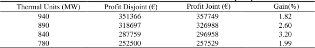
Finally, consider that each thermal unit power capacities are scaled down by the ratio given by the quotient of the thermal units installed capacity given in the first column of Table 3 by the initial installed capacity of 1440 MW. An equivalent conversion are performed on the ramp up/down, start-up and shutdown costs. The expected profit as a function of the thermal power installed capacity, keeping constant the wind power installed capacity, i.e., 360 MW, are shown in Table 3.

Table 3. Gain variation in function of thermal capacity

Thermal Units (MW) Profit Disjoint (€) Profit Joint (€) Gain(%)

940 351366 357749 1.82

890 318697 326988 2.60

840 287759 296958 3.20

780 252500 257529 1.99

Table 3 allows to conclude that the gain is dependent of the ratio between the wind power and the thermal power installed capacities. The maximum gain of 3.20% is achieved when the thermal power system installed capacity is about 2.3 times the wind power system installed capacity. Hence, there is not a fixed ratio between the wind power and the thermal power installed capacities that can be recommended independently of the power system total installed capacity.

4 Conclusion

Stochastic programming is a suitable approach to address parameter uncertainty in modelling via scenarios. Particularly, the stochastic MILP approach is well-known by being accurate and having greater computationally acceptance, since the CPU time scales up linearly with number of price scenarios, units and hours on the time horizon. The joint bid of thermal and wind power by a stochastic MILP approach proved to provide better expected profits than the disjoint bids. The expected profit is dependent in a nonlinear relation of the ratio between the wind power and the thermal power systems installed capacities.

The joint schedule is not a burden in computational resources in comparison with the disjoint one: the CPU time is about the same for both schedules, since the wind power system schedule CPU time is irrelevant when compared with the thermal power system one.

Acknowledgments. This work is funded by Portuguese Funds through the

Foundation for Science and Technology-FCT under the project LAETA 2015‐2020, reference UID/EMS/50022/2013; FCT Research Unit nº 151 C‐MAST Center for Mechanical and Aerospace Sciences and Technology.

(10)

References

1. Laia, R., Pousinho, H.M.I., Melício, R., Mendes, V.M.F.: Self-scheduling and bidding strategies of thermal units with stochastic emission constraints. Energy Conversion and Management, 89, 975–984 (2015)

2. Kongnam, C., Nuchprayoon, S.: Feed-in tariff scheme for promoting wind energy generation. In: IEEE Bucharest Power Tech. Conf., 1–6, Bucharest, Rumania (2009) 3. Bitar, E.Y., Poolla, K.: Selling wind power in electricity markets: the status today, the

opportunities tomorrow. In: American Control Conf., 3144–3147, Montreal, Canada (2012) 4. Barros, J., Leite, H.: Feed-in tariffs for wind energy in Portugal: current status and

prospective future. In: 11th Int. Conf. on Elec. Power Quality and Utilization, 1–5, Lisbon, Portugal (2011)

5. Al-Awami, A.T., El-Sharkawi, M.A.: Coordinated trading of wind and thermal energy. IEEE Transactions on Sustainable Energy, 2(3), 277–287 (2011)

6. Cena, A.: The impact of wind energy on the electricity price and on the balancing power costs: the Spanish case. In: European Wind Energy Conf., 1–6, Marceille, France (2009) 7. El-Fouly, T.H.M., Zeineldin, H.H., El-Saadany, E.F., Salama, M.M.A.: Impact of wind

generation control strategies, penetration level and installation location on electricity market prices. IET Renewable Power Generation, 2, 162–169 (2008)

8. Bathurst, G.N., Weatherill, J., Strbac, G.: Trading wind generation in short term energy markets. IEEE Transactions on Power Systems, 17, 782–789 (2002)

9. Matevosyan, J., Solder, L.: Minimization of imbalance cost trading wind power on the short-term power market. IEEE Transactions on Power Systems, 21, 1396–1404 (2006)

10. Pinson, P., Chevallier, C., Kariniotakis, G.N.: Trading wind generation from short-term probabilistic forecasts of wind power. IEEE Transactions on Power Systems, 22, 1148–1156 (2007)

11. Ruiz, P.A., Philbrick, C.R., Sauer, P.W.: Wind power day-ahead uncertainty management through stochastic unit commitment policies. In: IEEE/PES Power Syst. Conf. Expo., 1–9, Seattle, USA (2009)

12.Laia, R., Pousinho, H.M.I., Melício, R., Mendes, V.M.F.: Optimal bidding strategies of wind-thermal power producers. In: Technological Innovation for Cyber-Physical Systems, 394, Eds. Camarinha-Matos L.M., Falcão A.J., Vafaei N., Shirin Najdi P., 494–503 (2016) 13. Fan, S., Liao, J.R., Yokoyama, R., Chen, L.N., Lee, W.J.: Trading wind generation from

short-term probabilistic forecasts of wind power. IEEE Transactions on Power Systems, 24, 474–482 (2009)

14.Kusiak, A., Zheng, H., Song, Z.: Wind farm power prediction: a data-mining approach. Wind Energy, 12, 275–293 (2009)

15.Laia, R., Pousinho, H.M.I., Melicio, R., Mendes, V.M.F., Reis, A.H.: Schedule of thermal units with emissions in a spot electricity market. In: Technological Innovation for the Internet of Things, 394, Eds. Camarinha-Matos, L.M., Tomic, S., Graça, P., 361–370 (2015) 16.Catalão, J.P.S., Mariano, S.J.P.S., Mendes, V.M.F., Ferreira, L.A.F.M.: Short-term

electricity prices forecasting in a competitive market: a neural network approach. Electr. Power Syst. Res., 77, 1297–1304 (2007)

17.Coelho, L.D., Santos, A.A.P.: A RBF neural network model with GARCH errors: application to electricity price forecasting. Electr. Power Syst. Res., 81, 74–83 (2011) 18.Amjady, N., Daraeepour, A.: Mixed price and load forecasting of electricity markets by a

new iterative prediction method. Electr. Power Syst. Res., 79, 1329–1336 (2009)

19. Morales, J.M., Conejo, A.J., Ruiz, J.P.: Short-term trading for a wind power producer. IEEE Transactions on Power Systems, 25(1), 554–564 (2010)

20. Laia, R., Pousinho, H.M.I., Melício, R., Mendes, V.M.F., Collares-Pereira, M.: Spinning reverve and emission unit commitment through stochastic optimization. In: IEEE SPEEDAM, 444–448, Ischia, Italy (2014)