American Dairy Science Association, 2006.
The Accuracy of Seven Mathematical Functions in Modeling Dairy
Cattle Lactation Curves Based on Test-Day Records
From Varying Sample Schemes
A. M. Silvestre,1F. Petim-Batista, and J. Colac¸o
Departement of Animal Science–CECAV, University of Tra´s-os-Montes e Alto Douro, 5001-801 Vila Real, Portugal
ABSTRACT
Daily milk yield over the course of the lactation fol-lows a curvilinear pattern, so a suitable function is required to model this curve. In this study, 7 functions (Wood, Wilmink, Ali and Schaeffer, cubic splines, and 3 Legendre polynomials) were used to model the lactation curve at the phenotypic level, using both daily observa-tions and data from commonly used recording schemes. The number of observations per lactation varied from 4 to 11. Several criteria based on the analysis of the real error were used to compare models. The performance of models showed few discrepancies in the comparison criteria when daily or 4-weekly (with first test at days in milk 8) data by lactation were used. The performance of the Wood, Wilmink, and Ali and Schaeffer models were highly affected by the reduction of the sample dimension. The results of this work support the idea that the performance of these models depends on the sample properties but also shows considerable varia-tion within the sampling groups.
Key words: dairy cow, lactation curve INTRODUCTION
The modeling of lactation curves is not a new research topic. The first reference to a lactation curve model is attributed to Brody et al. (1924). Due to calculation difficulties and computer limitations, the first models of lactation curves were characterized as logarithmic transformations of exponential, polynomial, and other linear functions. At the end of the 1980s and during the 1990s, nonlinear models in the parameters were investigated (Grossman and Koops, 1988). Tozer and Huffaker (1999) characterized average lactation curves for Holstein-Friesian cows according to parity, whereas Tekerli et al. (2000) and Macciotta et al. (2005) studied the shape of lactation curve. Carta et al. (1995) studied the influence of seasonal effects on lactation curves of
Received January 2, 2005. Accepted November 8, 2005.
1Corresponding author: [email protected]
1813
dairy goats, and Groenewald et al. (1995) and Hohenbo-ken et al. (1992) investigated the suitability of mathe-matical models to represent the lactation curve of Me-rino sheep and beef cows, respectively.
Lactation curve models are an essential research tool for developing and validating mechanistic models, aimed at explaining the main features of the milk pro-duction pattern in terms of the known biology of the mammary gland during pregnancy and lactation (Neal and Thornley, 1983; Macciotta et al., 2005). The study of the mathematical properties of the lactation curve provides summarized information about dairy cattle production, which is useful in making management de-cisions (e.g., health monitoring, individual feeding). The models developed are also useful in the genetic analysis of test-day records to account for the effect of lactation stage (Ptak and Schaeffer, 1993) and to model the covar-iance between test-day records in a random regression analysis (Jamrozik and Schaeffer, 1997).
A variety of different mathematical models have been used in research on the shape of the lactation curve; this study compared the properties of 7 of these models. Wood’s (1967) curve (WOOD) has been used by a num-ber of researchers, most recently by Varona et al. (1998). The Wilmink (1987) model (WIL) was developed in the Netherlands and was the original function used to de-scribe the shape of the lactation curve in the official program of genetic evaluation of Canada (Schaeffer et al., 2000). The logarithm-based model developed by Ali and Schaeffer (1987; ALI) is also an important refer-ence that has been used in subsequent studies (Guo and Swalve, 1995; Jamrozik and Schaeffer, 1997). These 3 models have the common characteristic of being devel-oped specifically for lactation curves. Recently, scien-tists have begun to apply general mathematical tools, including splines and Legendre polynomials (White et al., 1999; Macciotta et al., 2005), to lactation curve modeling.
Current technologies allow the automatic measure-ment and recording of milk production at every milking. In this study, daily data of 144 lactations were used to achieve 8 sampling schemes, taking into account 4 intervals from calving to first test and 2 intervals
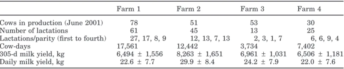
be-Table 1. Summary of daily data from 144 lactations for DIM interval 5 to 305
Farm 1 Farm 2 Farm 3 Farm 4 Cows in production (June 2001) 78 51 53 30
Number of lactations 61 45 13 25
Lactations/parity (first to fourth) 27, 17, 8, 9 12, 13, 7, 13 2, 3, 1, 7 6, 6, 9, 4
Cow-days 17,561 12,442 3,734 7,402
305-d milk yield, kg 6,494 ± 1,556 8,263 ± 1,651 6,961 ± 1,031 6,506 ± 1,181 Daily milk yield, kg 22.6 ± 7.7 29.9 ± 8.4 24.2 ± 7.9 22.0 ± 7.6
tween tests. The purpose of this work was to investigate the suitability of 7 mathematical functions in modeling the lactation curve from test-day records based on these different sampling schemes.
MATERIALS AND METHODS
Data
The data were obtained from May 1999 to June 2001, from 4 dairy farms with electronic identification and automatic milking recording systems. All farms were located in the north of Portugal. The number of milking cows when the last data recording was made is an indi-cator of farm dimension (Table 1). On all farms, cows were housed indoors, fed complete rations, and milked twice daily.
Software used on the farms allowed the storage of data from the most recent 60 milkings (30 daily milk yields) for management purposes. However, this pa-rameter was changed to allow the data store of 90 daily milk yields. The database used on this work had the daily milk yield of 144 complete lactations of 139 healthy cows; a total of 45,213 cow-days. Only 41,139 cow-days were considered in this study, however, be-cause records were restricted to those between 5 and 305 DIM. Some lactations had fewer than 305 d. Of the 144 lactations, 47, 39, 25, and 33 were first, second, third, and fourth lactations, respectively. Five cows had data from both first and second lactations. Overall means (± SD) for lactation length, total milk yield, and 305-d milk yield were 317± 50 DIM, 7,249 ± 1,892, and 7,091± 1,680 kg, respectively (Table 1).
For each lactation, 8 data sets of DIM were made according to the following criteria: 4 intervals from calv-ing to first test (8, 30, 60, and 90 d) and 2 intervals between tests (4 and 8 wk). Table 2 shows the adopted identification of the 8 sampling groups (SG; SG1 to SG8) and the mean number of observations per lacta-tion, which ranged from 4 to 11. Not all sampling groups had 144 lactations because a minimum of 4 observa-tions per lactation was required. In addition to these 8 data sets, all daily data were used to test how well the mathematical functions are able to model the lactation curves when all data are available (SG0).
Lactation Curve Models
Seven mathematical functions were applied to fit the milk yield data of individual lactations. The individual fit of lactation curves has been used in previous studies with the purpose of comparing functions or investigat-ing the effect of environmental factors such as herd, parity, and calving season on lactation curve traits (Tekerli et al., 2000; Rekik and Gara, 2004).
The Wood Model. The gamma function described by Wood (1967) is one of the most popular models used to describe the lactation curve:
Yt= atbe−ct. [1]
For all models, Ytis the milk yield in lactation day t.
In model [1], parameter a is a scaling factor to represent yield at the beginning of lactation, and parameters b and c are factors associated with the inclining and de-clining slopes of the lactation curve, respectively.
The Wilmink Model. The WIL model is the fol-lowing:
Yt= a + be−kt+ ct. [2]
According to Wilmink (1987), the parameters a, b, and c are associated with the level of production, the increase of production before the peak, and with the subsequent decrease, respectively. Parameter k is re-lated to the time of peak lactation and usually assumes a fixed value, derived from a preliminary analysis made on average production. This implies that the model has only 3 parameters to be estimated (Wilmink, 1987; Olori et al., 1999; Schaeffer et al., 2000). In a preliminary analysis, k was estimated at 0.065.
Ali and Schaeffer Model. The ALI model was pub-lished by Ali and Schaeffer (1987) in a work where the authors studied 3 lactation curve models with the objective of computing relative efficiencies of selection to change the shape of the lactation curve. This model can be written as follows:
Table 2. Identification of 8 sampling groups (SG) accordingly to sampling criteria, number of lactations,
and maximum number of observations per lactation.
Interval from calving to first test day Sampling
interval 8 d 30 d 60 d 90 d
4 wk SG1 (144; 11) SG2 (144; 10) SG3 (144; 9) SG4 (143; 8) 8 wk SG5 (144; 6) SG6 (142; 5) SG7 (137; 5) SG8 (134; 4)
where γt = t/305, Wt = ln (305 / t), a is a parameter
associated with the peak yield, d and e are parameters associated with increasing slope, and b and c are associ-ated with decreasing slope. The ALI has been consid-ered numerous times in studies applying test-day mod-els (e.g., Jamrozik and Schaeffer, 1997; Kettunen et al., 2000). In the present study, ALI was applied only in sampling schemes that yielded data from 7 or more observations per lactation. Consequently, this function was not fitted in SG6, SG7, and SG8 and was partially fitted in SG5, SG3, and SG4.
Cubic Splines Model. The smoothing cubic splines (SPL) is a semiparametric model recently used to de-scribe the lactation curve (White et al., 1999; Silvestre et al., 2005) and requires a minimum of 3 observations. The lactation is broken into separate periods, with spe-cific DIM identified as breakpoints between periods. A cubic spline is a piecewise cubic function that is con-strained so that the function and its first 2 derivatives are continuous at the breakpoints (knots) between one cubic segment (lactation period) and the next (White et al., 1999). Then, the model equation for each record can be written as:
yt= ai+ bi(t− ti) + ci(t− ti)2 [4]
+ di(t− ti)3, for ti≤ t ≤ ti+1.
According to Green and Silverman (1994), equation [4] represents the cubic polynomial for the interval be-tween the knots tiand ti+1with the 4 polynomial
coeffi-cients (ai, bi, ci, and di) for this cubic piece. To be one
cubic spline, equation [4] must satisfy conditions of con-tinuity between all the i knots (Green and Silverman, 1994; Verbyla et al., 1999). The SPL was applied to individual lactations using the program ASREML (Gil-mour et al., 2002). Verbyla et al. (1999) show that a smoothing cubic spline can be written as an estimated straight line (Xsβs) plus a predicted random effect
(Zsus). The number of equidistant knots on sampling
group SG0 was 32. On the other sampling groups, the number of knots varied from 11 (SG1) to 4 (SG8) and knotpoints were placed according to the same criteria described to achieve the sampling groups.
Legendre Polynomials Model. The Legendre poly-nomials (LEG) are polynomial functions of n degree
and domain n + 1 and the equation describing a single observation can be written:
Yt=
∑
ni=0
αiφi(w) [5]
where w is standardized unit of time ranging from −1 to +1, w = 2 t− tmin tmax− tmin − 1 [6]
and tmin(5 d) is the earliest DIM and tmax(305 d) is the
latest DIM (Schaeffer, 2004).
φn(w) =
√
2n + 1
2 Pn(w), [7]
where Pn(w) is a polynomial of degree n and φn(w) is
the normalized polynomial.
Normalized Legendre polynomials functions of stan-dardized units of time w and coefficients αiwith degree
2, 3, and 4 (LEG2, LEG3, and LEG4) were used in this study, and thus required a minimum of 4, 5, and 6 observations by lactation, respectively. The first 5 Leg-endre polynomials functions of standardized units of time (w) are defined below (equation 8), according to Spiegel (1971). P0(w) = 1 P1(w) = w P2(w) = 1 2(3w 2− 1) [8] P3(w) = 1 2(5w 3− 3w) P 4(w) = 1 8(35w 4− 30w2+ 3).
Comparison Criteria for the Models
The analysis of residuals is a common technique in the evaluation and comparison of models, in which a residual for a given record of daily yield is the difference between the observed value and the value predicted by the regression equation. However, the data used in this study allowed a more extensive examination, because all the daily yields between the sample dates were also known. This fact allowed us to not only evaluate errors
of estimation for the sample days, but to compare the lactation curves estimated by each of the functions with the real lactation curve for each cow. In this context, the error we evaluated was the mean real error (difference between the actual milk yield and estimated milk yield for every DIM, not just for those days corresponding to the sample dates). The following criteria were used, and were based DIM from 5 to 305:
a) Average and standard deviation of error. These criteria measure the error in absolute terms (Con-gleton and Everett, 1980; Guo and Swalve, 1995) without recognizing its variation through the lac-tation.
b) Correlation between the real milk yield and the estimated milk yield (R), which quantifies the de-gree of association between real and estimated val-ues (Guo and Swalve, 1995).
c) The quotient (Q) between the error sum of squares and the observed sum of squares. The quotient can be defined as follows: Q = 100
∑
305 i=5 e2 i∑
305 i=5 y2i [9]where yiis milk yield and eiis the error term.
Ac-cording to Ali and Schaeffer (1987), this criterion emphasizes the similarity between the real lacta-tion curve and the estimated lactalacta-tion curve. d) The Wald-Wolfowitz run test (W, nonrandom
dis-tribution for P< 0.05). The randomness of the dis-tribution of the errors is desirable and can be quan-tified, measured and tested by so-called run tests (Constantinides, 1988). The Wald-Wolfowitz run test is a nonparametric test that detects serial pat-terns in a run of numbers. Applied to the errors of each lactation, a significant test (P< 0.05) indicates the presence of sequences of positive or negative residuals longer than expected.
e) The Durbin-Watson statistic (D) is used to test for the presence of first-order autocorrelation in the errors. The test compares the error of DIM t with the error from DIM t − 1 and develops a statistic that measures the significance of the correlation between these successive comparisons (Seber and Wild, 1989). D =
∑
n i=2 (ei− ei−1)2∑
n i=1 (ei)2 [10]The statistic (D) is used to test for the presence of both positive and negative correlations among the errors. The Durbin-Watson statistic has a range from 0 to 4; D values near 2 indicate there is no correlation. When successive errors are close to each other, the D statistic will be near zero, sug-gesting the presence of positive autocorrelation. When successive errors are far from each other, the D value is near 4 suggesting the presence of negative autocorrelation. However, there exists an inconclusive region within which the D can fall and on which no interpretation can be made (Seber and Wild, 1989). Upper and lower bounds delineating those regions are defined according to tabulated critical values depending on the number of inde-pendent variables and on the number of observa-tions (Durbin and Watson, 1951).
f ) Percentage of estimated milk yields≤0 (EXLO) or >50 kg (EXHI). The 41,139 actual daily milk yields considered in the analysis had a mean of 24.8± 8.6 kg, and in only 58 cases were there values higher than 50 kg, corresponding to an expectation of 0.14%. Thus, all estimates of milk yield≤0 kg were considered to be biologically impossible and models were considered less reliable if the proportion of milk yield estimates>50 kg differed from 0.14%. Criteria a), b), and g) were calculated across all re-cords, whereas criteria c) and d) were calculated within lactations. Criterion e) was applied to the daily average values of each one of the 8 sampling groups (Table 1).
RESULTS
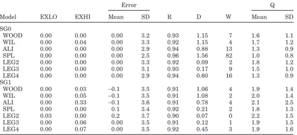
Comparative Study of the Models in SG0 and SG1 Seven mathematical functions were applied to fit the milk yield data of individual lactations with daily data (SG0) and in diverse circumstances of data availability. Although 8 sampling groups were considered (Table 2), SG1 was selected for more detailed discussion because it simulated the common situation of monthly test-day records (4-wk interval) and yielded the greatest number of observations per lactation. Results from sampling groups SG0 and SG1 are shown in Table 3. More simi-larity was observed among functions for SG0 than among the 8 sampling groups. In addition, all models fit the data more closely when all data were used (SG0) than when analyses relied on samples of data, as ex-pected. With SG0, no differences among functions were observed for EXLO, EXHI, and error average, with the exception of a nonzero EXHI for WIL. The proportion of lactations with random distribution of error was greater for SG0 than for analyses based on sampled
Table 3. Comparison criteria results of the Wood (WOOD), Wilmink (WIL), Ali and Schaefer (ALI), cubic
spline (SPL), and Legendre polynomial (LEG) models in sampling groups SG0 and SG1 for the 144 lactations1
Error Q
Model EXLO EXHI Mean SD R D W Mean SD
SG0 WOOD 0.00 0.00 0.00 3.2 0.93 1.15 7 1.6 1.1 WIL 0.00 0.04 0.00 3.3 0.92 1.15 4 1.7 1.2 ALI 0.00 0.00 0.00 2.9 0.94 0.88 13 1.3 0.9 SPL 0.00 0.00 0.00 2.5 0.96 1.56 82 1.0 0.8 LEG2 0.00 0.00 0.00 3.3 0.92 0.09 2 1.8 1.2 LEG3 0.00 0.00 0.00 3.1 0.93 0.17 9 1.5 1.0 LEG4 0.00 0.00 0.00 2.9 0.94 0.60 16 1.3 0.9 SG1 WOOD 0.00 0.03 −0.1 3.5 0.91 1.06 4 1.9 1.4 WIL 0.00 0.05 −0.1 3.5 0.91 1.08 2 2.0 1.4 ALI 0.00 0.33 −0.1 3.6 0.91 0.78 4 2.1 2.5 SPL 0.00 0.00 0.1 3.4 0.92 0.21 2 1.8 1.3 LEG2 0.03 0.00 0.2 3.7 0.90 0.07 0 2.2 1.5 LEG3 0.00 0.06 0.00 3.5 0.91 0.12 1 1.9 1.5 LEG4 0.00 0.07 0.00 3.5 0.92 0.45 3 1.9 1.6
1SG0 = Daily data; SG1 = 11 test days per lactation; EXLO = percentage of estimated milk yields lower
or equal to zero; EXHI = percentage of estimated milk yields higher than 50 kg; Error = difference between daily milk yield and estimated milk yield for every DIM; R = correlation between daily milk yield and estimated milk yield; D = Durbin-Watson test (positive autocorrelation) for D< 1.57); W = Wald-Wolfowitz test (number of lactations with random distribution); and Q = quotient between error sum of squares and observation sum of squares.
data and model SPL had the highest score (82 of 144 lactations with random distribution of errors). With regard to standard deviation of error, R, W, and Q, SPL ranked as the best model, followed by ALI and LEG4. Positive autocorrelation among errors was observed for all 7 models, but this property was least severe in SPL, WOOD, and WIL. In general, LEG2 yielded the poorest results for all of the comparison criteria.
Figure 1 shows the average error distribution in the range DIM 5 to 305. A common pattern was observed in the 7 models, in which average errors oscillated be-tween negative and positive during the lactation. For almost all DIM, errors were greatest (absolute value) for LEG2. The patterns found in Figure 1 suggest that the distribution of the errors, particularly for Legendre polynomials, was not random during lactation. This graphic illustration is supported by the results of the run test (W) and Durbin-Watson test presented in Table 3. The run test identified only a few lactations for each model with a random distribution of error, as W varied from 0 (LEG2) to 4 (WOOD, ALI). Positive autocorrela-tions were observed for all models, but Legendre polyno-mials and SPL had lower values for the Durbin-Watson test than the other 3 models. Although all models fit the data more closely for SG0 than SG1, the relative performance of the 7 functions did not show many dif-ferences in the comparison criteria across sampling groups SG0 and SG1.
Study of the Models’ Performance in Diverse Circumstances of Data Availability
Tables 4 and 5 summarize the performance of the various models in situations in which data were sam-pled bimonthly (SG5 to SG8) or when the first sample date occurred after the first month of lactation (all ex-cept SG5). Positive autocorrelations among errors were observed in all models. Moreover, in all the models, the run test results indicated that the distribution of the errors were predominantly nonrandom, with slight variation within functions and within sampling groups. For WOOD, no estimates of milk yield<0 occurred (Table 4). Numerous differences in the other compari-son criteria were observed across sampling groups. The standard deviation of error (>12.6), correlation between true and estimated yield (R< 0.53), and Q (x > 30; SD > 128) all suggested a poor fit in sampling groups SG3, SG4, SG7, and SG8. Poorer results were observed for SG3, with 9 test days per lactation, than for SG6, with 5 only observations per lactation. This fact seems to indicate that the problems were a consequence of the greater interval from calving to first test for SG3.
The results of the test criteria for WIL clearly showed inadequate performance in all the sampling groups when the first test day occurred at 60 or 90 DIM (Table 4). Thus, the efficiency of model WIL strongly depended on the length of the interval from calving to the first test day.
Figure 1. Distribution of average error (kg/d) for DIM 5 to 305 in sampling group SG1, and for Wood (WOOD), Wilmink (WIL), Ali and
Schaeffer (ALI), cubic splines (SPL), and Legendre polynomials (LEG2, LEG3, LEG4) functions.
The model ALI, with 5 parameters, is more de-manding than models WOOD and WIL, in terms of the minimum number of test-day records required per lactation, and its performance was acceptable only for the sampling groups SG1 and SG5. Standard deviation
of error, EXHI, R, and Q (Table 4) all tended to be excessively high, with problems increasing as the num-ber of sample days decreased and interval to first test-day increased. The highest scores for EXHI (1.38), error standard deviation (15.6), and Q ((x = 34.4; SD = 61.6),
Table 4. Comparison criteria results of the Wood (WOOD), Wilmink (WIL), Ali and Schaefer (ALI), and cubic spline (SPL) models in
sampling groups (SG) from SG2 to SG81
Error Q
Model/SG F I N n EXLO EXHI Mean SD R D W Mean SD
WOOD SG2 4 30 144 41,139 0.00 0.53 −0.2 4.3 0.88 0.36 3 3.0 4.5 SG3 4 60 144 41,139 0.00 1.62 −0.8 17.6 0.41 0.03 0 45 225 SG4 4 90 143 40,947 0.00 4.80 −19.3 367.1 0.04 0.10 0 445 2,011 SG5 8 8 144 41,139 0.00 0.06 0.0 3.8 0.90 1.17 2 2.3 2.3 SG6 8 30 142 40,759 0.00 0.55 −0.4 4.7 0.85 0.22 1 3.6 5.4 SG7 8 60 137 39,741 0.00 1.72 −0.8 12.6 0.53 0.03 1 30 128 SG8 8 90 134 39,057 0.00 4.07 −105 9764 0.00 0.29 0 799 4,949 WIL SG2 4 30 144 41,139 0.01 0.72 0.00 5.5 0.81 0.36 1 5.0 6.4 SG3 4 60 144 41,139 0.04 3.57 1.0 32.9 0.25 0.03 1 155 245 SG4 4 90 143 40,947 0.08 9.61 0.4 234.3 0.00 0.10 0 7,716 11,491 SG5 8 8 144 41,139 0.00 0.16 −0.1 3.8 0.90 1.17 2 2.2 1.7 SG6 8 30 142 40,759 0.01 0.88 −0.1 6.0 0.79 0.22 1 5.7 6.4 SG7 8 60 137 39,741 0.04 3.75 0.8 35.3 0.23 0.03 0 196 290 SG8 8 90 134 39,057 0.09 8.75 1.8 261.8 0.00 0.92 0 9,573 17,117 ALI SG2 4 30 144 41,139 0.01 1.38 0.2 15.6 0.45 0.07 1 34.4 61.6 SG3 4 60 142 40,759 0.06 4.77 3.3 112.7 0.08 0.06 1 1,891 3,261 SG4 4 90 136 39,517 0.10 8.11 22.2 391.5 0.02 0.02 0 23,225 30,455 SG5 8 8 100 29,853 0.00 0.71 0.1 5.1 0.82 0.58 0 4.1 5.8 SPL SG2 4 30 144 41,139 0.00 0.21 −0.4 3.7 0.91 0.05 4 2.2 1.4 SG3 4 60 144 41,139 0.00 0.64 −0.7 4.2 0.88 0.03 1 2.9 2.3 SG4 4 90 143 40,947 0.00 0.85 −1.0 4.8 0.86 0.02 1 3.8 3.6 SG5 8 8 144 41,139 0.00 0.00 0.5 4.0 0.89 0.08 1 2.5 2.1 SG6 8 30 142 40,759 0.00 0.21 −0.5 4.0 0.89 0.06 3 2.6 1.7 SG7 8 60 137 39,741 0.00 0.48 −0.5 4.4 0.87 0.04 1 3.1 2.3 SG8 8 90 134 39,057 0.00 0.53 −0.8 5.0 0.83 0.03 1 4.1 4.0
1F = Frequency of sampling (wk); I = interval from calving to first test day (d); N = number of lactations; n = number of lactation
cow-days; EXLO = percentage of estimated milk yields lower or equal to zero; EXHI = percentage of estimated milk yields higher than 50 kg; Error = difference between daily milk yield and estimated milk yield for every DIM; R = correlation between daily milk yield and estimated milk yield; D = Durbin-Watson test (positive autocorrelation) for D< 1.57); W = Wald-Wolfowitz test (number of lactations with random distribution); and Q = quotient between error sum of squares and observation sum of squares.
and the lowest correlation values (R = 0.45) in the study were all obtained for the model ALI.
The SPL model seemed to be the least sensitive to changes in test-day interval and time between calving and first test-day. This result may be due to the particu-larities of this semiparametric model. With SPL, no estimates of negative milk yield occurred and cases of EXHI were<1%. These were the best results observed for those 2 criteria. Results achieved across sampling groups for average and standard deviation of error (<1 and≤5, respectively), correlation (R > 0.83), and Q (x < 4.1; SD < 4.0) were considerably better for SPL than for WOOD, WIL, and ALI (Table 4).
The Legendre polynomials (Table 5) did not show much variation in the comparison criteria across sam-pling groups and were more suitable for describing the lactation curve when the first test day was recorded late in lactation than were WOOD, WIL, and ALI (Table 4). However, models LEG2, LEG3, and LEG4 required at least 4, 5, and 6 test-day records in each lactation, respectively, which implies that they were not
applica-ble to all the sampling groups. When comparing the Legendre polynomials with each other for EXHI, stan-dard deviation of error, R, and Q, model LEG2 ranked highest in model fit, followed by LEG3 and LEG4 for SG2, SG3, SG4, SG6, and SG7. However, this order was reversed for SG5.
DISCUSSION
When monthly test-day data (with the first test at DIM 8) were used, all 7 functions described the lactation curve with similar accuracy. Differences in goodness of fit between functions became more visible with reduc-tion of data availability. Accuracy of models WOOD, WIL, and ALI was particularly affected by increasing the interval between tests. The fit of these 3 models was also compromised when the interval between calv-ing and the first test day increased. When the first test occurred after 2 mo of lactation, the best models for fitting the lactation curve were the nonparametric mod-els (SPL and LEG), with an advantage for the SPL.
Table 5. Comparison criteria results of the Legendre (LEG) polynomials in sampling groups from SG2 to
SG81
Error Q
Model/SG F I N n EXLO EXHI Mean SD R D W Mean SD LEG2 SG2 4 30 144 41,139 0.04 0.30 −0.40 3.80 0.90 0.06 1 2.3 1.6 SG3 4 60 144 41,139 0.00 0.69 −0.64 4.53 0.87 0.03 2 3.4 3.6 SG4 4 90 143 40,947 0.02 1.72 −1.07 5.93 0.79 0.02 0 6.8 17.2 SG5 8 8 144 41,139 0.11 0.00 0.50 4.13 0.88 0.05 1 2.7 2.5 SG6 8 30 142 40,759 0.03 0.27 −0.33 4.11 0.89 0.07 0 2.8 2.1 SG7 8 60 137 39,741 0.04 0.45 −0.56 4.58 0.86 0.03 2 3.4 2.5 SG8 8 90 134 39,057 0.18 1.52 −0.97 5.97 0.79 0.03 3 6.0 6.5 LEG3 SG2 4 30 144 41,139 0.00 0.34 −0.4 3.9 0.90 0.08 1 2.4 1.9 SG3 4 60 144 41,139 0.00 1.19 −0.6 5.3 0.83 0.04 0 4.4 4.8 SG4 4 90 142 40,759 0.01 3.78 −1.1 10.0 0.60 0.02 0 17.1 27.6 SG5 8 8 135 39,290 0.00 0.00 0.2 4.0 0.88 0.10 1 2.5 2.5 SG6 8 30 134 39,057 0.00 0.22 −0.5 4.5 0.86 0.08 1 3.2 2.6 SG7 8 60 105 31,257 0.00 0.86 −0.2 5.2 0.82 0.08 1 4.4 4.5 LEG4 SG2 4 30 144 41,139 0.00 0.36 −0.3 4.0 0.89 0.20 2 2.6 2.4 SG3 4 60 142 40,759 0.01 1.92 −0.1 8.5 0.69 0.38 2 11.6 22.3 SG4 4 90 136 39,517 0.04 4.37 0.9 20.0 0.33 0.03 0 66.1 99.7 SG5 8 8 100 29,853 0.00 0.00 0.3 3.7 0.89 0.35 0 2.2 2.1
1F = Frequency of sampling (wk); I = interval from calving to first test day (d); N = number of lactations;
n = number of lactation cow-days; EXLO = percentage of estimated milk yields lower or equal to zero; EXHI = percentage of estimated milk yields higher than 50 kg; Error = difference between daily milk yield and estimated milk yield for every DIM; R = correlation between daily milk yield and estimated milk yield; D = Durbin-Watson test (positive autocorrelation) for D< 1.57); W = Wald-Wolfowitz test (number of lactations with random distribution); and Q = quotient between error sum of squares and observation sum of squares.
Moreover, SPL had the additional advantage of describ-ing the lactation curve adequately with fewer observa-tions than required for ALI, LEG3, and LEG4. The results obtained for LEG on SG3, SG4, SG7, and SG8 can be explained by the greater flexibility of orthogonal polynomials compared with parametric models (Macci-otta et al., 2005). The same argument has been pre-viously presented for cubic splines by White et al. (1999).
In sampling group SG2, ALI was the worst of all the functions, according to the criteria used in this study. The sampling groups SG1 and SG2 coincide with the collecting criteria of the Portuguese test-day data. Re-sults attained by ALI on SG2 indicate that this model is the least adequate for application to test-day data with these properties. The sampling groups SG3 and SG4 had more tests per lactation than did SG5 and SG6. Even so, all 7 functions achieved better results with SG5 and SG6 than with SG3 and SG4. These results confirm the importance of data collection during the initial phase of lactation. The availability of test-day records before the peak yield is crucial for correct estimation of lactation curve shape (Kellogg et al., 1977; Macciotta et al., 2005). According to Rekik and Gara (2004), the probability of occurrence of atypical curves increases by 4% for each day that the first test-day date is delayed.
Variation in fit of the various functions was observed among cows, among models, and among sampling groups. The variation in fit among cows within the same sampling group illustrated by the Q values suggests that the suitability of the models considered depends not only on the mathematical form of the function, but also on individual trends in daily milk yield, which vary among cows and among lactations of the same animal. The ability to capture all of this information depends on the amount of data available and on its distribution during lactation. This individual variation has been observed in previous studies but was attributed to the effects of several environmental and genetic factors (Perochon et al., 1996). Lactation curve traits are also affected by environmental variables such DIM at first test day, calving age, calving year, calving season, par-ity, and pregnancy status (Tekerli et al., 2000; Rekik and Gara, 2004). The lactation curve has also been studied at the genetic and permanent environmental levels (Kettunen et al., 2000). However, Olori et al. (1999) analyzed data from a uniform group of cows from the same herd and, even under these conditions, the variation in fit was almost entirely among cows rather than between their tested models.
The increasing pressure to reduce costs associated with milk recording schemes is a reality in several coun-tries (Liu et al., 2000) and it has also become noticeable
in Portugal. In such a situation, models with the proper-ties of model SPL and Legendre polynomials (i.e., abil-ity to fit the data with increasing intervals between test days) must be investigated, as well as their application on test-day models for genetic evaluation.
CONCLUSIONS
Considering daily data, SPL and functions with 5 parameters (ALI and LEG4) showed superior fit to the data, although the performance of all models was ac-ceptable. Differences among models became more pro-nounced as the amount of data decreased and timing of the initiation of data collection was delayed. In partic-ular, the performance of WOOD, WIL, and ALI models were strongly affected by the reduction of the sample dimension, especially with an increase in the interval between calving and the first test day. The results of this work support the idea that the performance of the considered models depends on the sampling properties, but high variability among individual cattle was ob-served within sampling schemes. Because widespread implementation of a milk recording scheme that collects data with more than a monthly frequency may not be economically feasible, research to define adequate mod-els for the lactation curve will continue to be necessary.
ACKNOWLEDGMENTS
Authors wish to acknowledge the 2 anonymous refer-ees for their helpful comments and suggestions.
REFERENCES
Ali, T. E., and L. R. Schaeffer. 1987. Accounting for covariances among test day milk yields in dairy cows. Can. J. Anim. Sci. 67:637–644. Brody, S., C. W. Turner, and A. C. Ragsdale. 1924. The relation between the initial rise and subsequent decline of milk secretion following parturition. J. Gen. Physiol. 6:541–545.
Carta, A., S. R. Sanna, and S. Casu. 1995. Estimating lactation curves and seasonal effects for milk, fat and protein in Sarda dairy sheep with a test day model. Livest. Prod. Sci. 44:37–44.
Congleton, J. R., and R. W. Everett. 1980. Application of the incom-plete gamma function to predict cumulative milk production. J. Dairy Sci. 63:109–119.
Constantinides, A. 1988. Applied Numerical Methods with Personal Computers. 2nd ed. McGraw-Hill, New York, NY.
Durbin, J., and G. S. Watson. 1951. Testing for serial correlation in least squares regression. Biometrika 30:159–178.
Gilmour, A. R., B. J. Gogel, B. R. Cullis, S. J. Welham, and R. Thomp-son. 2002. ASReml User Guide Release 1.0. VSN International Ltd., Hemel Hempstead, UK.
Green, P. J., and B. W. Silverman. 1994. Nonparametric Regression and Generalized Linear Models. A Roughness Penalty Approach. Chapman & Hall, London, UK.
Groenewald, P. C. N., A. V. Ferreira, H. J. Van Der Merwe, and S. C. Slippers. 1995. A mathematical model for describing and predicting the lactation curves of Merino ewes. Anim. Sci. 61:95–101.
Grossman, M., and W. J. Koops. 1988. Multiphasic analysis of lacta-tion curves in dairy cattle. J. Dairy Sci. 71:1598–1608.
Guo, Z., and H. H. Swalve. 1995. Modelling of the lactation curve as a sub-model in the evaluation of test day records. Proc. Interbull Mtg. Prague, Czechoslovakia. International Bull Evaluation Ser-vice, Uppsala, Sweden. Interbull Bull. No. 11.
Hohenboken, W. D., A. Dudley, and D. E. Moody. 1992. A comparison among equations to characterize lactation curves in beef cows. Anim. Prod. 55:23–28.
Jamrozik, J., and L. R. Schaeffer. 1997. Estimates of genetic parame-ters for a test day model with random regressions for yield traits of first-lactation Holsteins. J. Dairy Sci. 80:762–770.
Kellogg, D. W., N. S. Urquhart, and A. J. Ortega. 1977. Estimating lactation curves with a gamma curve. J. Dairy Sci. 55:1308–1315. Kettunen, A., E. A. Mantysaari, and J. Poso. 2000. Estimation of genetic parameters for daily milk yield of primiparous Ayrshire cows by random regression test-day models. Livest. Prod. Sci. 66:251–261.
Liu, Z., R. Reents, F. Reinhardt, and K. Kuwan. 2000. Approaches to estimating daily yield from single milk testing schemes and use of a.m.-p.m. records in test-day model genetic evaluation in dairy cattle. J. Dairy Sci. 83:2672–2682.
Macciotta, N. P. P., D. Vicario, and A. Cappio-Borlino. 2005. Detection of different shapes of lactation curve for milk yield in dairy cattle by empirical mathematical models. J. Dairy Sci. 88:1178–1191. Neal, H. D., and J. H. M. Thornley. 1983. The lactation curve in cattle: A mathematical model of the mammary gland. J. Agric. Sci. (Camb.) 101:389–400.
Olori, V. E., S. Brotherstone, W. G. Hill, and B. J. McGuirk. 1999. Fit of standard models of the lactation curve to weekly records of milk production of cows in a single herd. Livest. Prod. Sci. 58:55–63.
Perochon, L., J. B. Coulon, and F. Lescourret. 1996. Modelling lacta-tion curves of dairy cows with emphasis on individual variability. Anim. Sci. 63:189–200.
Ptak, E., and L. R. Schaeffer. 1993. Use of test day yields for genetic evaluation of dairy sires and cows. Livest. Prod. Sci. 34:23–34. Rekik, B., and A. B. Gara. 2004. Factors affecting the occurrence of
atypical lactations for Holstein–Friesian cows. Livest. Prod. Sci. 87:245–250.
Schaeffer, L. R. 2004. Application of random regression models in animal breeding. Livest. Prod. Sci. 86:35–45.
Schaeffer, L. R., J. Jamrozik, G. J. Kistemaker, and B. J. Van Door-maal. 2000. Experience with a test-day model. J. Dairy Sci. 83:1135–1144.
Seber, G. A. F., and C. J. Wild. 1989. Nonlinear Regression. John Wiley & Sons, Inc., New York, NY.
Silvestre, A. M., M. F. Petim-Batista, and J. Colac¸o. 2005. Genetic parameter estimates for milk, fat and protein using a spline test-day model. J. Dairy Sci. 88:1225–1230.
Spiegel, M. R. 1971. Advanced Mathematics for Engineers and Scien-tists. McGraw-Hill, New York, NY.
Tekerli, M., Z. Akinci, I. Dogan, and A. Akcan. 2000. Factors affecting the shape of lactation curves of Holstein cows from the Balikesir province of Turkey. J. Dairy Sci. 83:1381–1386.
Tozer, P. R., and R. H. Huffaker. 1999. Mathematical equations to describe lactation curves of Holstein-Friesian cows in South Wales. Aust. J. Agric. Res. 50:431–440.
Varona, L., C. Moreno, L. A. Garcia-Cortes, and J. Altarriba. 1998. Bayesian analysis of Wood’s lactation curve for Spanish dairy cows. J. Dairy Sci. 81:1469–1478.
Verbyla, A. P., B. R. Cullis, M. G. Kenward, and S. J. Welham. 1999. Smoothing splines in the analysis of designed experiments and longitudinal data. Appl. Stat. 48:269–311.
White, I. M. S., R. Thompson, and S. Brotherstone. 1999. Genetic and environmental smoothing of lactation curves with cubic splines. J. Dairy Sci. 82:632–638.
Wilmink, J. B. M. 1987. Adjustment of test-day milk, fat and protein yield for age, season and stage of lactation. Livest. Prod. Sci. 16:335–348.
Wood, P. D. P. 1967. Algebraic model of the lactation curve in cattle. Nature 216:164–165.