J. Microw. Optoelectron. Electromagn. Appl. vol.16 número3

(1)

DOI: http://dx.doi.org/10.1590/2179-10742017v16i3895

Brazilian Microwave and Optoelectronics Society-SBMO received 17 Jan 2017; for review 19 Jan 2017; accepted 07 Jun 2017 

Abstract—The numerical mode-matching (NMM) technique is a very efficient approach to analyze well-logging tools used for hy-drocarbon exploration. This problem is typically modeled as a cylindrically layered medium (subterranean formation) including both horizontal and vertical stratifications. In this paper, we present a new NMM formulation based on the use of B-splines expansion func-tions with variable knot multiplicity to represent the dependency of fields on the vertical direction, and cylindrical Bessel funcfunc-tions to represent the fields along the radial (horizontal) direction. We show that this type of expansion allows to better capture the spatial variation of the electromagnetic field near vertical layer interfaces. Illustrative examples elucidate the advantage of knot multiplicity in the modeling of earth formations with anisotropic and lossy layers. A case study on compensated dual resistivity (CDR) well-logging tool sensors is also presented based on the proposed method.

Index Terms—Numerical mode-matching, cubic B-splines, well-logging tools, compensated dual resistivity.

I. INTRODUCTION

OGGING-WHILE-DRILLING (LWD) tools are electromagnetic sensors routinely used to estimate constitutive parameters (permittivity and conductivity) of subterranean formations [1]. This information is useful is assessing the potential for hy-drocarbon bearing zones.

Continual advances in computing power have enabled the use of brute-force numerical techniques such as finite-differences (FD) [2–5] and finite volumes (FV) [7] to model LWD tools operating in complex geophysical environments. However, it is still impractical to employ brute-force methods in inversion efforts where a large number of forwards simulation is required for a parameter space sweep. On the other hand, methods that combine both numerical and analytical steps [8–13], such as the numer-ical mode-matching (NMM) [14–17], are able to model complex geophysical formations while requiring only a modest amount of computational resources compared to brute-force methods.

In this paper, we present a new NMM formulation based on the use of cubic B-splines with variable knot multiplicity to ex-pand the fields along the vertical direction. The knot multiplicity of these basis functions allow a better representation of the field behavior across interfaces while using a coarser computational grid, leading to a lesser demand on computational resources.

The remaining of this work is organized as follows. Section II summarizes the proposed formulation of NMM using cubic B-splines. Section III shows numerical results to validate the technique, drawing attention to some advantages of the proposed modal expansion based on multiple knots. Section IV presents a case study on compensated dual resistivity (CDR) well-logging tools. Finally, Section V provides some concluding remarks.

II. NUMERICAL MODE-MATCHING FORMULATION

The geometry of this problem can be adequately described in terms of a cylindrically layered medium composed of both radial (horizontal) and vertical stratifications [17]. In the NMM formulation presented in [15], the electromagnetic field is expanded in terms of basis functions that depend on the vertical coordinate z, while reflection and transmission matrices (obtained by enforc-ing the appropriate boundary conditions across interfaces) are used to represent the dependency along the radial coordinate ρ in terms of Bessel and Hankel functions.

This work was supported in part by the Brazilian Agencies CAPES and CNPq under doctoral fellowships 2444/11-9 and 150454/2016-3.

M. S. Canabarro is with the Center for Telecommunications Studies, Department of Electrical Engineering, Pontifical Catholic University of Rio de Janeiro, Rio de Janeiro, RJ 22451-900, Brazil (e-mail: [email protected]).

J. R. Bergmann is with the Center for Telecommunications Studies, Department of Electrical Engineering, Pontifical Catholic University of Rio de Janeiro, Rio de Janeiro, RJ 22451-900, Brazil (e-mail: [email protected]).

F. L. Teixeira is with the ElectroScience Laboratory, Department of Electrical and Computer Engineering, Ohio State University, Columbus, OH 43212, USA (e-mail: [email protected]).

A Numerical Mode-Matching Method Based on

Multiple-Knot Cubic B-Splines Applied to the

Analysis of Well-Logging Tools

Maiquel S. Canabarro, José R. Bergmann, and Fernando L. Teixeira

Centro de Estudos de Telecomunicações

–

PUC RIO, Brazil

[email protected]

(2)

Brazilian Microwave and Optoelectronics Society-SBMO received 17 Jan 2017; for review 19 Jan 2017; accepted 07 Jun 2017 A. Radial NMM

Assuming a time-harmonic dependence for the fields and sources in the form exp(i t), we obtain the two vector wave equa-tions for the electric and magnetic fields, respectively, as [6]



1



2 _{, and}

   

h E h E i hJ

      (1)



1



2 1

,

 

    

h H h H h J

       (2)

where the (anisotropic) constitutive properties of the medium are represented by the permittivity and permeability tensors,



and  [12,15]. The impressed electrical current J is produce by horizontal coil antennas wrapped around a metallic mandrel with radius_T. In addition, we assume the antennal to be axially located at z . Using a cylindrical coordinate system _T ( , , )  z aligned with the tool axis, the fields given in (1) and (2) can be represented by means of the Bessel transforms [18] as

1 ( , , ) ( , ), 2 iv v v

F

 

z e f



z











(3)

0

1

( , ) ( , ) ( ) ,

2

v v v

f  z f k_ z J k_ k dk_ _







_

(4)

where J_v(k_) is a Bessel function of order v , and f k_v( _, )z is the Hankel transformation of f_v( , )



z . Using (1), (3) and (4), we can rewrite (1) in terms of the z component of the electric field for a source-free region as

 

2 2 1 1 , 0 _ _   _  _  _ _ 

 h zv

v v

k d k z

z z



 





(5)

where d_z



_{v z}e is the electric flux density, which is expanded in a set of B-splines functions S z : _n( )

 

1

, .

zv z n n

n

d k_ z d z a S z





 



(6)

The substitution of (6) in (5) results in

 

2 2

1 1

,

n h n n n

n v n v

a w S z k a S z

z



z







 

 

 _{ }  _

_ _ 

 



(7)

where in practice, the series are truncated using a sufficient number of terms for a given grid resolution. The resulting problem can be arranged in a matrix form as

2 _.

n n

L_a_ k p_{ } a_ (8) Equation (8) represents a generalized eigenvalue problem where 2

k_ are the eigenvalues and a are the eigenvectors. Note that that matrices L_ and p_are symmetric in reciprocal media (i.e., with symmetric



and  ).

In regions with sources, the z-component of the fields obey the following equation:

 

2 1 2 2 1 , , ,

v v v v z

h v z

d z

z z

i j z

                   _ _   _  _  _ _ _ _ 

  (9)

where the electric flux density is given by the expansion:

 

   

1

, ,

N

z q q

q

d  z b   z





(10)

 

1

.





N

q q _n n

n

a S z



(11)

(3)

prod-DOI: http://dx.doi.org/10.1590/2179-10742017v16i3895

Brazilian Microwave and Optoelectronics Society-SBMO received 17 Jan 2017; for review 19 Jan 2017; accepted 07 Jun 2017 uct along z, we find

 









2 2 2 1 1 , q q

T q T

k b j                  _{  }  _  _ _        (12)

where jTq represents the spectral contribution of the source for the TE modes. Note that only TE modes are excited by

hori-zontal coil antennas as considered here.

B. Transimpedance Calculation

With the expressions of the fields in the source region, we can now obtain the values of the induced voltages at a given receiv-er coil due to a current in the transmittreceiv-er antenna. The transimpedance is defined as

1

,

  R 

_



RT R

T T

V

Z E dl

I I (13)

Where, since the receiver coil antennas are horizontal, we only need to consider the azimuthal electric field component. The latter can be written in the following form [6]:

 

, t

 

,

R R

E_  z S z _  (14) where

 

1 1 1,0 1 1 1

1 1 1 1 1,2 1

T T

R

T T

Y H R Y J d

Y H Y J R d

                  _ _ _ _ _ _          _ _ _ _ _ __ _    (15)

is a factor depending on the reflection coefficients across layers. See [15] for more details on the evaluation of (13). C. Cubic B-Spline Eigenfunctions

In the NMM formulations described in [6] and [19], the electromagnetic fields were approximated by triangular, sinusoidal and quadratic B-splines basis functions. In the present work, we adopt cubic B-splines as base (expansion) functions [20] be-cause of their high-order nature and ability to handle knots of higher multiplicity. The function Sn

 

z employed in (6) can be

each written as a combination of four polynomial terms:

 

 1

 

 2

 

 3

 

 4

 

,

n

S z Seg z Seg z Seg z Seg z (16)

where

 

102 3

1

30 20

,

 z

Seg z u

z z (17)

 

102 21 10 212 2

2

30 20 30 20 30 20

2 2 2

3

21 21 21

30 20 30 31 41 31

3 3 ,                  _   _  

z z z z

Seg z u u

z z z z z z

z z z

u

z z z z z z

(18)

 

32 20 42 21 322 21 32

3

30 31 41 31 30 31 41 31

2 2 2 2 2

2 3

32 32 32 32 32

30 31 41 31 30 31 41 31 41 42

3 3 ,     _  _ _  _                    

z z z z z z z

Seg z u

z z z z z z z z

z z z z z

u u

z z z z z z z z z z

(19)

 

₄₃2

 

3

4

41 42

1 ,

 z 

Seg z u

z z (20)

(4)

Brazilian Microwave and Optoelectronics Society-SBMO received 17 Jan 2017; for review 19 Jan 2017; accepted 07 Jun 2017

10 1 0 40 4 0

21 2 1 41 4 1

1

2 1

... ,

. i

i i

z z z z z z

z z u

z z



 

   

 



(21)

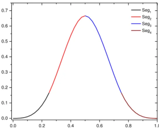
Each B-spline has five knots (nodes). When these knots are equally spaced, we obtain a uniform B-spline, as shown in in Fig. 1.

0.0 0.2 0.4 0.6 0.8 1.0

0.0 0.1 0.2 0.3 0.4 0.5 0.6

0.7 Seg₁

Seg2

Seg₃

Seg4

Fig. 1. The four polynomials that compose a uniform cubic B-spline with five equally space knots.

When two or more knots are collocated in space, we obtain a knot with higher multiplicity. Fig. 2 illustrates the behavior of a cubic B-spline function for different knot multiplicities. The top curve shows a case with single knots only. The mid curve shows a case with one knot with double multiplicity. The bottom curve shows a case with one knot with triple multiplicity. By increas-ing the multiplicity, one decreases the regularity of the function. At the knot with double multiplicity the cubic B-spline has dis-continuous second derivative, whereas at the knot with triple multiplicity the cubic B-spline has disdis-continuous first derivative. This properties allows for properly capturing the behavior of the electromagnetic fields from the boundary conditions across layer interfaces.

Fig. 2. Cubic B-spline behavior for different knot multiplicities.

III. THE KNOTS-MULTIPLICITY EFFECTS

In order to first examine the effect of the multiplicity of knots of the cubic B-splines functions in a simpler setting, we consid-er the problem of a parallel plate guide filled by two layconsid-ers in the z-direction, as shown in Fig. 3. This problem admits an analyti-cal solution as described in [21]. The eigenvalues for TM and TE (to z ) waves satisfy

2 2 2

0, and

 v 

z v

h

k_  k  k

 (22)

2 2 2 0 ,

 h  z

k_



k k (23)

(5)

Brazilian Microwave and Optoelectronics Society-SBMO received 17 Jan 2017; for review 19 Jan 2017; accepted 07 Jun 2017 above with the values predicted by (22) and (23).

Fig. 3. Parallel plate waveguide filled with two vertical layers.

A. Isotropic and Lossless Layers

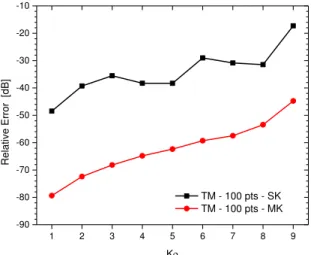
Consider a scenario with d  1000 m and a  500 m, as indicated in Fig. 3. The upper layer has ₁ ₀ and  ₁ ₀and the bottom layer has ₂ 2.55₀ and  ₂  ₀. The relative error in the solution of the radial wavenumber k_ for the first 9 modes with expansions using multiple knots (MK) or only single knots (SK) are depicted in Fig. 4 and Fig. 5, for the TM and TE fields, respectively. We can observe that lower order modes present a significant reduction by using MK. The differences be-tween the MK and SK results are more pronounced for TM modes. This behavior can be explained by the presence of a double derivative with respect to z in the first term within the brackets in (7). In this case, the MK expansion provides, of course, a more accurate result compared to the SK expansion.

1 2 3 4 5 6 7 8 9

-90 -80 -70 -60 -50 -40 -30 -20 -10

Relative

Erro

r

[dB]

K

TM - 100 pts - SK TM - 100 pts - MK

(6)

1 2 3 4 5 6 7 8 9

-110 -100 -90 -80 -70 -60 -50 -40 -30

Relative

Erro

r [

dB]

K

TE - 100 pts - SK TE - 100 pts - MK

Fig. 5. Relative error on TE eigenvalues, in the case of isotropic and lossless layers.

B. Isotropic and Lossy Layers

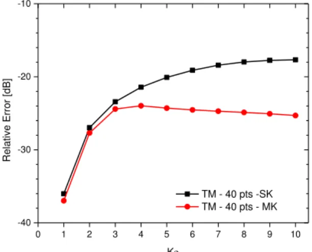
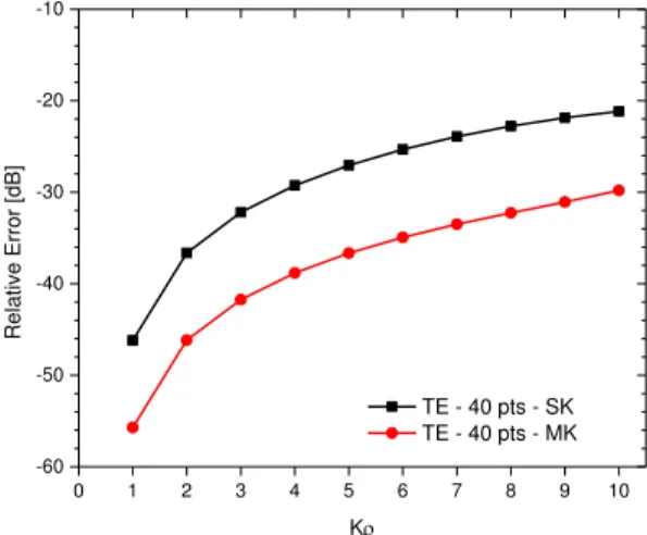
As a second example, consider now a parallel plate waveguide filled with lossy layers. Layer 1 has  ₁ ₀ and ₁ 1 S/m, and layer 2 has  ₂ ₀ and ₂ 100 S/m. In addition the vacuum permeability is present everywhere. The distance between the plates is now d 20 m. Fig. 6 and Fig. 7 present the relative error in the solution of k_ for the first 10 modes with MK and SK. We again observe smaller errors by using MK compared to SK, for both TM and TE modes.

0 1 2 3 4 5 6 7 8 9 10

-40 -30 -20 -10

Relative

Erro

r [

dB]

K

TM - 40 pts -SK TM - 40 pts - MK

Fig. 6. Relative error on TM eigenvalues, in the case of isotropic and lossy layers.

0 1 2 3 4 5 6 7 8 9 10 -60

-50 -40 -30 -20 -10

Relative

Erro

r [

dB]

K

TE - 40 pts -SK TE - 40 pts - MK

(7)

Brazilian Microwave and Optoelectronics Society-SBMO received 17 Jan 2017; for review 19 Jan 2017; accepted 07 Jun 2017 C. Anisotropic and Lossy Layers

In a third example, consider uniaxially anisotropic and lossy layers. The upper layer has 1, ,v h 0 and 1,v 1 S/m and 1,h 100 S/m

  . The bottom layer has _{2, ,}v h ₀, 2,v 100 S/m and 2,h  1 S/m. Again, we consider d20 m. Fig. 8 and

Fig. 9 show results for the first ten modes using SK and MK, for both TM and TE modes, respectively. Once more, the ad-vantage of the MK approach is clear compared to SK.

0 1 2 3 4 5 6 7 8 9 10

-80 -70 -60 -50 -40 -30

Relative

Erro

r [

dB]

K

TM - 40 pts - SK TM - 40 pts - MK

Fig. 8. Relative error on TM eigenvalues, in the case of anisotropic and lossy layers.

0 1 2 3 4 5 6 7 8 9 10 -60

-50 -40 -30 -20 -10

Relative

Erro

r [

dB]

K

TE - 40 pts - SK TE - 40 pts - MK

Fig. 9. Relative error on TE eigenvalues, in the case of anisotropic and lossy layers.

IV. CASE STUDY: BOREHOLE WITH RUGOSITY

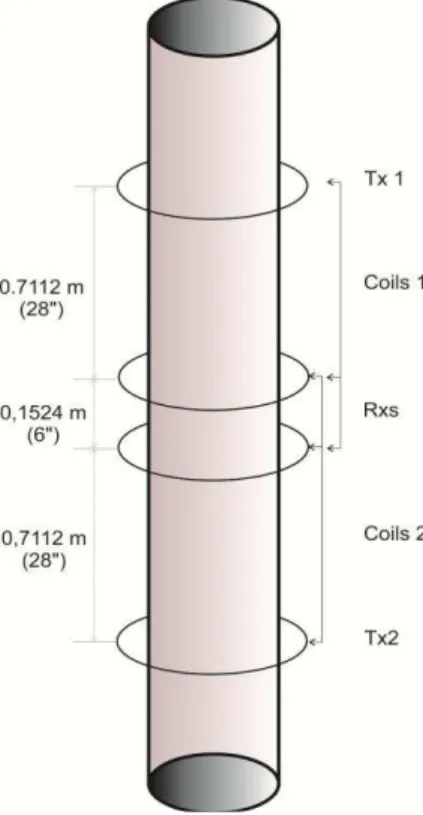
Next, we consider a compensated dual-resistivity (CDR) LWD tool traversing a rugose borehole. This problem was considered before in [22, 23] and is examined here to validate our formulation and illustrate the ability of the proposed algorithm based on MK cubic B-splines to efficiently model this kind of problem. The CDR sensor operates at 2MHz and is composed by two transmitters and two receivers as depicted in Fig. 10. Typically, this sensor yields two apparent resistivities, Rps and Rda,

asso-ciated with the phase difference and the amplitude ratio of the voltage inducted at the receiver antennas. The Rps resistivity

pro-vides information of radial regions close to the antennas while the R_da resistivity provides information from regions farther from the antennas.

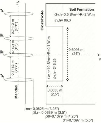
The transmitters and receivers are modelled as coil antennas with radius of 3.5 in. The conductor mandrel is modeled as a PEC cylinder with radius of 3.25 in. The sensor antennas are placed concentrically around the mandrel, and their axial positions are represented in Fig. 10. The CDR sensor moves along a 2.5-in-rugose borehole wall, as depicted in Fig. 11, inside a

(8)

Brazilian Microwave and Optoelectronics Society-SBMO received 17 Jan 2017; for review 19 Jan 2017; accepted 07 Jun 2017 [22, 23].

To eliminate spurious reflections arising from the truncation of the domain along z, we employed a cylindrical perfectly matched layer with properties similar to that used in [24]. Initially, we use a uniform grid along z with  z 0.020 m within the domain of interest and based on SK. The resistivity results due to transmitter 2 excitation are shown in Fig. 12 (note that, in this uncompensated case, transmitter 1 is not active). The abscissa axis represents the midpoint between the two receivers, i.e.,



zr1zr2



/ 2. We can clear see that the rugosity in the borehole wall disturbs the response of the sensor resistivity compared to the smooth wall solution. This can lead to misinterpretations when reading the LWD sensor response.

(9)

Brazilian Microwave and Optoelectronics Society-SBMO received 17 Jan 2017; for review 19 Jan 2017; accepted 07 Jun 2017 Fig. 11. CDR sensor tool inside a rugose borehole.

0 1 2 3 4 5 6

0.5 1 10

[



.m]

(Z_r1+Z_r2)/2 [m]

Rda - Uncompensated - NMM Rps - Uncompensated - NMM

Fig. 12. Amplitude and phase apparent resistivities of a CDR sensor tool due the transmitter 2 alone (uncompensated).

(10)

0 1 2 3 4 5 6

0.5 1 10

[



.m]

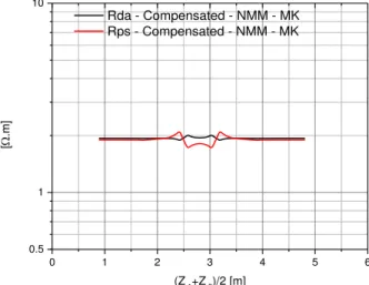
(Zr1+Zr2)/2 [m] Rda - Compensated - NMM - MK Rps - Compensated - NMM - MK

Fig. 13. Amplitude and phase apparent resistivities of a compensated CDR sensor tool modeled by the NMM employing MK cubic B-splines.

V. CONCLUSION

We have introduced a new NMM formulation based on the use of cubic B-splines with multiple knots as expansion functions, for the modeling of well-logging tools. Numerical results showed that the use of knots with higher multiplicity allows for a better representation of the fields near interface layers of typical geophysical scenarios. The presented technique is able to accurately model complex media including anisotropic and lossy layers using less grid points than conventional (uniform) cubic B-splines. As such, the proposed technique represents a useful improvement on the modeling of well-logging-tools.

REFERENCES

[1] S. Y. Chen, W. C. Chew, V. R. N. Santos, K. Sainath, and F. L. Teixeira, “Electromagnetic subsurface remote sensing,” in: Wiley Encyclopedia of

Electri-cal and Electronics Engineering, John Wiley & Sons, New York, 2016.

[2] Y.-K. Hue, F. L. Teixeira, L. San Martin, and M. Bittar, ‘Three-dimensional simulation of eccentric LWD tool response in boreholes through dipping

formations,’ IEEE Trans. Geosci. Remote Sens., vol. 43, no. 2, pp. 257-268, 2005.

[3] H.O. Lee and F. L. Teixeira, ‘Cylindrical FDTD analysis of LWD tools through anisotropic dipping layered earth media,’ IEEE Trans. Geosci. Remote

Sens., vol. 45, no. 2, pp. 383-388, 2007.

[4] D. Wu, C. R. Liu, and J. Chen, “An efficient FDTD method for axially

symmetric LWD environments,” IEEE Trans. Geosci. Remote Sens.,

vol. 46, no. 6, pp. 1652–1656, 2008.

[5] H. O. Lee, F. L. Teixeira, L. E. San Martin, and M. S. Bittar, `Numerical modeling of eccentered LWD borehole sensors in dipping and fully anisotropic Earth formations,' IEEE Trans. Geosci. Remote Sens., vol. 50, no. 3, pp. 727-735, 2012.

[6] M. S. Novo, L. C. Silva, and F. L. Teixeira, `Three-dimensional finite-volume analysis of directional resistivity logging sensors,’ IEEE Trans. Geosci.

Remote Sens., vol. 48, no. 3, pp. 1151-1158, 2010.

[7] M. S. Novo, L. C. da Silva and F. L. Teixeira, “Finite volume modeling of borehole electromagnetic logging in 3-D anisotropic formations using coupled scalar-vector potentials,” IEEE Antennas Wireless Propag. Lett., vol. 6, pp. 549-552, 2007.

[8] J. R. Lovell and W. C. Chew, “Response of a point-source in a multicylindrically layered medium,” IEEE Trans. Geosci. Remote Sens., vol. 25, no. 6, pp. 850–858, 1987.

[9] J. R. Lovell and W. C. Chew, “Effect of tool eccentricity on some electrical well-logging tools,” IEEE Trans. Geosci. Remote Sens., vol. 28, no. 1, pp. 127–

136, 1990.

[10] Z.-Q. Zhang and Q.-H. Liu, “Applications of the BCGS-FFT method to 3-D induction well-logging problems,” IEEE Trans. Geosci. Remote Sens., vol. 41, no. 5, pp. 998–1004, 2003.

[11] Y.-K. Hue and F. L. Teixeira, ‘Analysis of tilted-coil eccentric borehole antennas in cylindrical multilayered formations for well-logging applications,’

IEEE Trans. Antennas Propaga t., vol. 54, no. 4, pp. 1058-1064, 2006.

[12] G.-S. Liu, F. L. Teixeira, and G.-J. Zhang, `Analysis of directional logging tools in anisotropic and multieccentric cylindrically-layered Earth formations,'

IEEE Trans. Antennas Propagat., vol. 60, no. 1, pp. 318-327, 2012.

[13] H. Moon, B. Donderici, and F. L. Teixeira, `Stable evaluation of Green’s functions in cylindrically stratified regions with uniaxial anisotropic layers,’ J.

Comp. Phys., vol. 325, pp. 174-200, 2016.

[14] G.-X. Fan, Q. H. Liu, and S. P. Blanchard, “3-D numerical mode-matching (NMM) method for resistivity well-logging tools,” IEEE Trans. Geosci. Remote Sens., vol. 38, no. 10, pp. 1544–1552, 2000.

[15] Y.-K. Hue and F. L. Teixeira, 'Numerical mode-matching method for tilted coil antennas in cylindrically layered anisotropic media with multiple horizontal

beds,’ IEEE Trans. Geosci. Remote Sens., vol. 45, no. 8, pp. 2451-2462, 2007.

[16] W. C. Chew, Waves and Fields in Inhomogeneous Media. New York, NY, USA: John Wiley & Sons, 1995.

[17] J. Li and L. C. Shen, “Vertical eigenstate method for simulation of induction and MWD resistivity sensors,” IEEE Trans. Geosci. Remote Sens., vol. 31, no. 2, pp. 399-406, Mar. 1993.

[18] E. Cavanagh and B. Cook, “Numerical evaluation of Hankel transforms via Gaussian-Laguerre polynomial expansions,” IEEE Trans. Acoustics, Speech,

Signal Proc., vol. 27, no. 4, pp. 361-366, Aug. 1979.

(11)

[20] H. Yang, W. Yue, Y. He, H. Huang, and H. Xia, “The deduction of coefficient matrix for cubic non-uniform B-Spline curves,” in 1st Int. Workshop Edu.

Technol. Comp. Sci., Hubei, China, pp. 607-609, 2009.

[21] R. F. Harrington, Time-Harmonic Electromagnetic Fields. New York, NY, USA: McGraw-Hill, 1961.

[22] B. Clark., M. G. Luling, J. Jundt, M. O. Ross, and D. L. Best, “A dual depth resistivity measurement for FEWD,” in SPWLA 29th Annual Logging Symp., paper SPWLA-1988-A, San Antonio, TX, USA, 5-8 June, 1988.

[23] B. Clark., D. F. Allen, D. L. Best, S. D. Bonner, J. Jundt, M. G. Luling, and M. O. Ross, “Electromagnetic propagation logging while drilling: Theory and

experiment,” SPE Format. Eval., vol. 5, no. 3, pp. 263-271, 1990.

[24] F. L. Teixeira and W. C. Chew, “Finite-difference computation of transient electromagnetic waves for cylindrical geometries in complex media,” IEEE