277
COMPLEX FUNCTIONS WITH GEOGEBRA
Ana Maria d’Azevedo Breda and José Manuel Dos Santos Dos SantosUniversidade de Aveiro, Instituto GeoGebra, Portugal ambreda@ua.pt, dossantosdossantos@gmail.com
Complex functions, generally feature some interesting peculiarities, seen as extensions real functions, complementing the study of real analysis. However, the visualization of some complex functions properties requires the simultaneous visualization of two-dimensional spaces. The multiple Windows of GeoGebra, combined with its ability of algebraic computation with complex numbers, allow the study of the functions defined from ℂ to ℂ through traditional techniques and by the use of Domain Colouring. Here, we will show how we can use GeoGebra for the study of complex functions, using several representations and creating tools which complement the tools already provided by the software. Our proposals designed for students of the first year of engineering and science courses can and should be used as an educational tool in collaborative learning environments. The main advantage in its use in individual terms is the promotion of the deductive reasoning (conjecture / proof). In performed the literature review few references were found involving this educational topic and by the use of a single software.
Keywords: Complex Functions, Domain Colouring, Visualization, GeoGebra
INTRODUCTION
In Visual complex analysis Tristan Nendhan tell us how in the last one hundred years the bourbakista view of mathematics led to the “divorce from one’s sensory experience of the world, despite the fact that the very phenomena one is studying were often discovered by appealing to geometric (and perhaps physical) intuition.” (Nenglam, 1997, p.vii).
Nenglam (1997) is one of the mathematicians who tries to reverse this situation, making even appeal to the use of computers to visualize mathematical objects. For Nenglam mathematicians must think computers “as a physicist would his laboratory – it may be used to check existing ideas about the construction of the world, or as a tool for discovering new phenomena which then demand new ideas for their explanation (Nenglam, 1997, p.viii)
In an attitude of perfect agreement with Nendham ideas is Vieira Alves, who explains his attempt to illustrate the Fundamental Theorem of Algebra (Vieira Alves, 2013). He uses the features of GeoGebra 2D and the Maple’s CAS and 3D capabilities. Of course, the use of single software for the features mentioned is an added value. The great advantage of using 3D GeoGebra is just this. Although the need to carry out further literature review, for this type of mathematical content and having in mind educational purposes and their application with groups of students, we found references to MatLab, used in the context of simulation problems (Meng, Jiang, Shi, & Liang, 2014). Another study was conducted by Yong-Ming and Dan mentions the use of computational tools to calculate integrals of complex functions and they still refer mathematical experiences with students from collaborative nature. It should be pointed out that these studies are focus in mathematical calculations and about visualization issues and don’t use GeoGebra. However, the GeoGebra was used in a research with a control group as a tool in collaborative and cooperative learning environments, in spite of being embedded in a real analysis context (Takači, Stankov, & Milanovic, 2015).
278
Starting from several examples of complex functions, in the first section of this article, we illustrate various forms to represent such functions, contributing to the understanding of their geometric properties and how they can be viewed as extensions of real functions. One of the strategies used to analyse some properties of complex functions is the exploration/visualization of the behaviour of the image set by a complex function of affixes of complex points on subset of points in the domain. Within this purpose, it were developed for GeoGebra tools creating some particular type of grids in a Graphics window of GeoGebra, representing the function domain, at the same time, the image of the grid by the function is visualized in a Graphics 2 window. In fact, the graphical windows of GeoGebra correspond to the Cartesian representations of ℝ2, isomorphic to ℂ, being models of excellence for the representation of the domain and codomain of the function that we want to analyze. Being the GeoGebra software that allows the user interaction with geometric and algebraic properties simultaneously, the possibility of moving points on particular subsets of the domain, allows us to stimulate the students view by their assessment to instantaneous images of the image set of these points, allowing conjectures about properties of complex functions of complex variable. In the second section of this article, we will use the 3D capabilities of GeoGebra to analyze the real part and the imaginary part of a complex function, as a strategy to deepen the analysis of complex functions of complex variable. GeoGebra has a 3D graphic window which leads to the possibility to obtain an immediate graphical representation of the components of the complex function (Breda, Trocado, & Santos, 2013). There is an increased interest in the use of GeoGebra to the teaching and learning of complex analysis considering representations of the domain and the codomain of complex functions, the graphic representation of their components and the interaction between distinct representations.
Another way to represent functions from ℂ to ℂ, or from ℝ2 to ℝ2, is the use of the so-called colouring domain technique. This will be focussed in the third section of this paper.
The colouring domain is a procedure popularized by Frank Farris (1997), previously used by Larry Crone and Hans Lundmark, is based on the use of a spectrum of colours that act as elements of replacement of the not accessible dimension and it was used to represent complex functions of complex variable. Thus, applying this technique using GeoGebra (Breda et al., 2013) we will obtain graphic representations of complex functions, weaving some considerations about the information obtained by the analysis of these graphics.
Finally, it will be presented some considerations about the capabilities of GeoGebra for the analysis of complex functions. We will also presented some clues and concerns for the development of future work, in particular, on the implementation of this technological device to the study of other properties of complex functions, as well as its potential in the teaching and learning processes of elementary complex analysis.
GRAPHIC WINDOWS OF GEOGEBRA AND GEOMETRIC REPRESENTATION OF COMPLEX FUNCTIONS
One of the strategies to analyse properties of a complex function, f, is given by considering a subset of the domain of the function, G ⊂ Df ⊆
ℂ
, and analysing the properties of the image set, f(G)⊆ℂ
. In general, the subsets are chosen to be Cartesian grids, however with GeoGebra is possible to use a wider set of domain subsets. In a first approach several tools were built allowing, through some279
parameters, to obtain some particular type of grids (table 1).
Tool name: CircleConcentric Grid RayConcentricGri d QuadrangularCon centricGrid EccentricityConce ntricGrid PointConcentricG rid Command
name: CCgrid RCgrid QCgrid ECgrid PCgrid Parameters : n=Slider[1, 10, 1, 1,100, false, true, false, false ] P=1+i d=Slider[0, 4, 0.1, 1,100, false, true, false, false ] n=Slider[1, 10, 1, 1,100, false, true, false, false ] P=1+i n=Slider[1, 10, 1, 1,100, false, true, false, false ] P=1+i d=Slider[0, 4, 0.1, 1,100, false, true, false, false ] n=Slider[1, 10, 1, 1,100, false, true, false, false ] P=1+i d=Slider[0, 4, 0.1, 1,100, false, true, false, false ] n=Slider[1, 10, 1, 1,100, false, true, false, false ] P=1+i d=Slider[0, 4, 0.1, 1,100, false, true, false, false ] Code: CC=Sequence[Circl e[(real(P),imaginar y(P)) , k d / n], k, 1, n, 1] RC=Sequence[Rota te[Segment[(real(P) , imaginary(P)), (real(P)) + d, imaginary(P))], i 2 π / n, (real(P), imaginary(P))], i, 0, n, 1] QC= {Circle[P, d], Sequence[Translate [Segment[P - d sqrt(2) / 2 (1, 1), P - d sqrt(2) / 2 (-1, 1)], (0, i d sqrt(2) / n)], i, 0, n, 1], Sequence[Translate [Segment[P - d sqrt(2) / 2 (1, 1), P + d sqrt(2) / 2 (-1, 1)], (d i sqrt(2) / n, 0)], i, 0, n, 1]} EC={Circle[P,d],Se quence[(x - real(P))² / (i d / n)² + (y - imaginary(P))² / (1 - 1 / (i d / n)²) = 1, i, 0, n, 1]} Sequence[Sequence [P + sqrt(2) d k / 2 + sqrt(2) ί d j / 2, k, -1, 1, sqrt(2) d / n], j, -1, 1, sqrt(2) d / n] Icon:
Purpose: Given P (in Argand
plane) d, and n. The tool draw a family of circles with centre in P and radius multiple of d/n.
Given P (in Argand plane) d, and n. The tool draw a family of Rays cantered at P, with length d and making
2 π / n as a minimum angle.
Given P (in Argand plane) d, and n. The tool draw an orthogonal gird with 2n segments centred at P and in-script in a circle with centre in P and radius d.
Given P (in Argand plane) d, and n. The tool draw a family of conics centred at P with eccentricity d/n and making 2 π / n as a minimum angle.
Given P (in Argand plane) d, and n. The tool draw an squared orthogonal gird with points centre in P and in-script in a circle centre in P and radius d.
Table 1. Tools that create subsets of points in the Argand plane
Let us assume that we wanted to study the function f: ℂ →ℂ: f (z) = z2. The classical geometric analysis uses the images by f of a subset of points in the complex plane. Using the tools presented in table 1, one we obtain the images illustrated in Figure 1. Handling the mobile point on the girds the user obtain relevant information about the behaviour of the complex function f (z)=z2 [2]. Looking at the first image of Figure 1 we can see a quadrangular concentric grid centred at 0+0i and a circle. The handling process leads, to the observation that circles of radius r, � =r, are sent to circles of radius r2, �=r2, and straight lines strictly parallel to the real and imaginary axes are sent to parables.
Besides, the real axis is sent to the positive real axis and the imaginary axis is sent to the real negative axis.
280
The second image, in Figure 1, allows you to strengthen the conjecture about the circles centred at the origin and displays that the family of six segments that make minimum angles of a sixth of 180 are sent in three segments which form an angle of at least one-third of 180, it seems so to say that the ray θ=k are sent by f in the ray of equation θ=2k. In the third image we can conjecture that ellipses are sent to ellipses and hyperbolas in parables.
Figure 1. Tools that create subsets of points in the Argand plane and their images by f: ℂ→ ℂ, f(z)=z2. The visualization and handling of the applications built with the GeoGebra display properties of this function, providing moments for conjectures and acting as facilitators to the mathematical proof. Note that here we have chosen a function allowing the realization of conjectures with a very simple evidence. Using other functions we may provide circumstances where the first strategy points toward a conjecture that is refuted by the analysis of their component functions (Breda et al., 2013: 80).
281
3D GRAPHIC WINDOWS OF GEOGEBRA AND REPRESENTATION OF THE COMPONENTS FUNCTIONS OF A COMPLEX FUNCTION
Considering the function used in the previous section we can easily obtain their components graphs. So considering z=x+yi, with x∈ ℝ and y∈ ℝ, the components of f are the functions: If(z)=2xy and Rf(z)=x2-y2. In GeoGebra we can represent the graph of functions of two variables, we can write the real component as f1(x,y)=real((x+yi)2) and the imaginary component as f2(x,y)=imaginary
((x+yi)2). In alternative we can also write f1(x,y)=x2-y2 and f2(x,y)=2x, in any case their graphic representations correspond to hyperbolic paraboloids (see fig. 2).
Figure 2. Graphical representation of components functions to f: ℂ → ℂ, f (z)=z2, on the left the function component corresponding to real part and, on the right, the corresponding to imaginary part. To analyse the image of a Cartesian grid we note that on the hyperbolic paraboloid, the image of the real part of the straight lines correspond to parables, i.e., the intersection of the surface defined by z=x2-y2 with planes with equation x=k or y=k are parables. The intersection of the planes of equation x=k or y=k with the hyperbolic paraboloid is not easily visualized, it seems to be straight lines, but observing carefully the algebraic expression of the imaginary part of the function, we may easily conclude that these are straight lines satisfying the equations x=k ∧ z=2ky or y=k ∧ z=2kx.
GEOGEBRA AND COLOURING DOMAINS IN REPRESENTATION OF THE GRAPH OF A COMPLEX FUNCTION
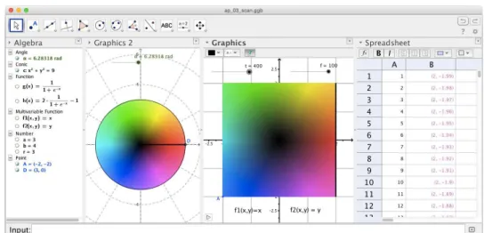
The technique of the colouring domain was implemented in Geiger by the authors of this paper in 2013, based on a preliminary work of Rafael Losada. In this technique each point has an associated and the colouring is done according to certain rules (Breda et al., 2013, p. 78). In the production of a colouring domain in GeoGebra a geometric scanning supported by values calculated in the spreadsheet is used, the colour of a point is given according to a given criterion, and the representation obtained can be contained in the Graphic windows (Breda et al., 2013) or Graphics 3D Windows (Breda & Santos, 2015). In Figure 3 is shown the application that generates the colouring domain of the identity function, the functions g and h which are crucial in the criterion for colouring domain, are visible in the algebraic window.
282
Figure 3. Application creating the scan of a colourful two-dimensional domain in GeoGebra.
The interest in the colouring domains is the representation of four dimension objects in a bi-dimensional colourful world, where the colour has a very important meaning. The colouring of the identity function gives us the starting point to gather information about the action of the function in study. Dark areas represent an approximation to zero and areas with a lot of brightness indicate the proximity of the pole of the Riemann sphere, i.e. values approaching infinity. In Figure 4 we can see the coloured areas associated with the complex functions j(z)=zeiθ. Looking at the images we may induce that these functions represent rotations of the complex plane.
f (z) =z2 I(z) =z j (z) =z ei π /4 j (z) =z ei π /2 j (z) =z ei 3π /4 j(z) =z ei π
Figure 4. Colouring Domain f (z) = z2 , of identity and
� � = z��, � ∈ {π /4, π /2, 3π /4, π }. Let us, now focus our attention on the first two images shown in Figure 4. On the left, comparing the colouring domain of the function f(z)=z2 with the colouring of the identity function, you will see the modification of the above mentioned angle duplication, the colour spectrum is repeated. Besides, an increase of the module by the function f, is also visible, the luminosity increases as we move away from the central point, at the same time, the dark zone close to zero also increases.
283
In fact, the search of zeros of a complex function is one of the situations where the use of the colouring domain is particularly suitable.
In Figure 6, looking at the colouring of the complex functions f(z)=z2 and l(z)=(z3-1)/z, z∈ ℂ
provided by GeoGebra, the perception of the zeros of these functions is very clear. In the case of f it corresponds to z=0+0i, in the case of the function l we may identify its zeros which correspond to the three roots of the unity in ℂ.
CONCLUSIONS
In the last few pages, we summarize the work done that so far with the purpose of studying complex functions using colouring domains developed in GeoGebra. We can say that this software allow the junction of several available mathematical resources with the ability to produce various graphical representations. The GeoGebra graphic capacities still need to be improved. With the GeoGebra current versions are still slow, especially in representations of 3D colouring domains. On the other hand the exploitation and dissemination of these applications are essential so that, this powerful tool can get to where it is most needed – to "classrooms". The knowledge about the role of the visualization in teaching and learning complex elementary analysis is still very incipient. The use of GeoGebra in this topic is still very fresh, however we have exposed that it is possible to make use of several representations to support the study, from multiple views, of some properties of complex functions.
NOTES
1. The GeoGebra version used in the applications referenced in this paper is 5.0.64.0-3D, February 13, 2015. However, these applications were created with version 4.9.183, December 21, 2013.
2. Note that � = ���� � and so �2= �2��� 2� , where �=|z|.
ACKNOWLEDGMENT This work was supported in part by Portuguese funds through the CIDMA (Center for Research and Development in Mathematics and Applications, and the Portuguese Foundation for Science and Technology (FCT-Fundação para a Ciência e a Tecnologia), within project PEst-OE/MAT/UI4106/2014. D. Kapanadze is supported by Shota Rustaveli National Science Foundation within grant FR/6/5-101/12 with the number 31/39
REFERENCES
Breda, A., Trocado, A., & Santos, J. (2013). O GeoGebra para além da segunda dimensão. Indagatio Didactica, 5(1). Retrieved from http://revistas.ua.pt/index.php/ID/article/view/2421, acceded at 15/02/2015. ISSN: 1647-3582
Breda, A., & Santos, J. (2015). The Riemann Sphere in GeoGebra. Sensos-e, 2(1). Retrieved from http://sensos-e.ese.ipp.pt/?p=7997, acceded at 15/02/2015. ISSN 2183-1432.
Farris, F. (1997). Visualizing Complex-valued Functions in the Plane. Retrieved from:
http://www.maa.org/pubs/amm_complements/complex.html , acceded at 15/02/2015.
Meng, P. C., Jiang, Z. X., Shi, S. Z., & Liang, S. M. (2014, June). Study of a Combination of Complex Function Learning with Mathematical Modeling. In 2014 International Conference on Management Science and Management Innovation (MSMI 2014). Atlantis Press.
Needham, T. (1997). Visual complex analysis. Oxford: Clarendon Press.
Poelke, K. & Polthier, K. (2009). Lifted Domain Coloring. Computer Graphics Forum, Oxford, v.28, n. 3, p. 735-742. Retrieved from: http://www.mi.fu-berlin, acceded at 15-02-2015.
284
Takači, D., Stankov, G., & Milanovic, I. (2015). Efficiency of learning environment using GeoGebra when calculus contents are learned in collaborative groups. Computers & Education, 82, 421-431.
Vieira Alves, F. R. (2013). Viewing The Roots of Polynomial Functions in Complex Variable: The Use of GeoGebra and The CAS Maple. Acta Didactica Napocensia, 6(4).
Wegert E. & Semmler G. (2011), Phase plots of complex functions: a journey in illustration. Notices Amer. Math. Soc. 58, 6, 768-780. Retrieved from: http://arxiv.org/pdf/1007.2295.pdf , acceded at 15-02-2015.
Zhang, Y. M., & Wang, D. (2013, June). Teaching Reform on The Course of Complex Analysis. In 2013 Conference on Education Technology and Management Science (ICETMS 2013). Atlantis Press.