1
Introduction
Based on the evidence collected by the research on neurosciences, Brocas and Carrillo (2008) and Alonso et al. (2014), have proposed to model the brain as an organization with peculiar features. These features include specialization (there are di¤erent brain systems, each one dedicated to a di¤erent task), centralization (a central executive system –CES –is responsible for a judicious allocation of scarce cognitive resources) and communication of needs (each system triggers a signal every time it requires resources to undertake a task).
The mentioned principles support the view that decision-making should be interpreted as an agency problem, where brain systems are the ‘agents’requiring resources to perform tasks and the CES assumes the role of ‘principal’, taking the responsibility of optimally allocating the available mental resources.
In the referred literature, the resource allocation problem is interpreted as being static. At a given point in time, an individual has a series of tasks to perform and the allocation of resources to each deliberative process will depend on the complexity of each task and on the resources it demands. Here, resource allocation in the brain is transformed into an intertemporal optimization problem, for which it is feasible to analyze the steady-state behavior and stability properties.
The adoption of a dynamic setting implies conceiving a choice problem in which the decision-maker is systematically faced, period after period, with the same set of tasks, such that the allocation of cognitive resources will converge towards a long-term equilibrium position where it tends to rest unless some external disturbance occurs.
The dynamic setup reveals some suggestive results. First, the steady-state will correspond to an array of resource shares e¢ ciently allocated to each system. Second, available resources might not be fully used; from an optimality perspective, some cognitive resources may fail to be allocated to the execution of any of the tasks. Third, the saddle-path stability result indicates that as long as the brain systems are able to communicate their needs to the CES, convergence to the long-run locus is attainable.
The remainder of the paper is organized as follows. Section 2 describes the agency prob-lem. Section 3 is dedicated to the analysis of the model’s dynamics. Section 4 concludes and highlights possible pathways for future research.
2
The Dynamic Agency Problem
Assume a decision-maker endowed with a …xed amount of cognitive resources, , which can be reused in every time period of the planning problem. Let there be n brain systems, each one associated with the ful…lment of a speci…c task i 2 N = f1; 2; :::; ng. For each brain system, a state variable !i(t)is de…ned; this represents the share of mental resources allocated to system i at date t. One also de…nes, again for each brain system, a control variable, i(t), which respects to the resources employed by system i in order to communicate needs to the CES.
Consider that the utility obtained from the execution of tasks in each brain system is a linear function of the allocated resources, i.e., U (!i(t) ) = u!i(t) , u > 0.1
1One could consider a ceiling on the resources required to execute each task, e
i, what would imply
U (!i(t) ) = u!i(t) for !i(t) ei and U (!i(t) ) = uei for !i(t) > ei. Without the ceiling one is
Assuming an in…nite horizon and a constant intertemporal discount rate, > 0, the aggre-gate objective function of the decision-maker is
(0) = M ax i(t);i2N 1 Z 0 " u X i !i(t) X i i(t) # exp( t)dt (1)
The individual intends to maximize the utility accomplished with solving tasks in the brain systems, while minimizing the resources spent by each one of the systems in transferring infor-mation on the task to the central brain unit. Optimization problem (1) is subject to a series of resource constraints that deliver the motion of !i(t);8i 2 N.
The amount of resources allocated to system i increases with the output of a matching function that has, as arguments, the system’s e¤ort variable and the overall amount of cognitive resources yet to be allocated,
yi(t) = f ( i(t); " 1 X j2N !j(t) # ) ; i2 N (2) De…nition 1Function f (:) : R2
+ ! R+ is a matching function of the dynamic agency problem if the following properties hold,
i) f is continuous and di¤erentiable;
ii) f is an increasing function in both arguments: f > 0, f(1 !) > 0;
iii) f is subject to decreasing marginal returns, for each of its inputs: f < 0, f(1 !) ;(1 !) < 0;
iv) f is homogeneous of degree 1, f ( i(t); " 1 X j2N !j(t) # ) = f ( i(t); " 1 X j2N !j(t) # ) ;8 > 0;
v) Both inputs are essential for resource allocation, f ( 0; " 1 X j2N !j(t) # ) = f [ i(t); 0] = 0:
The matching function indicates that when deliberating how much resources to attribute to each brain system, the CES simultaneously considers the signalling e¤ort made by the system and the amount of cognitive resources that are not yet employed in any of the considered system activities. The last property is particularly meaningful because it indicates that resource availability and the signalling of needs are both indispensable for a transference of resources to occur.
Besides increasing with the outcome of the matching process, the resources allocated to each system i will also su¤er the in‡uence of an automatic withdrawal by the CES; at each time period, the CES withdraws cognitive resources from each brain system at a constant rate 2 (0; 1). This translates the idea that the CES will progressively ignore system i unless the
ones available are fully allocated.
brain system is capable of keeping the attention of the CES by maintaining the value of i(t) persistently at a positive level.
With the previous information in mind, the resource constraints of the allocation problem are generically presentable as,
[!i(t) ] = yi(t) !i(t) ; !i(0)2 (0; 1) given, i 2 N (3) An explicit functional form for the matching function that obeys the properties in de…nition 1 is the Cobb-Douglas speci…cation,
yi(t) = Ai[ i(t)] (" 1 X j2N !j(t) # )1 ; i2 N; Ai > 0; 2 (0; 1) (4) In the above formulation, it is assumed that each matching process, for each brain system, has not necessarily the same e¢ ciency, i.e. the value of parameter Ai might vary across systems.
Under matching function (4), constraint (3) is equivalent to
!i(t) = Ai i(t) " 1 X j2N !j(t) #1 !i(t); !i(0)2 (0; 1) given, i 2 N (5) De…nition 2The dynamic agency problem (DAP), de…ned to characterize resource allocation in the brain, consists in solving (1) subject to: (i) equation (3) or, for an explicit Cobb-Douglas matching function, equation (5); and (ii) the constraints on state and control variables, 0 !i(t) 1and i(t) 0;8i 2 N.
3
Optimal Solution, Steady-State and Stability
The application of Pontryagin’s principle allows for a straightforward examination of the DAP. A …rst result concerns the optimal motion of the problem’s variables.
Proposition 1 Under conditions of optimality and considering the Cobb-Douglas matching function, the intertemporal behavior of the DAP is fully translated in the 2n dimensional system of di¤erential equations !i(t) = A 1=(1 ) i h pi(t) i =(1 )" 1 X j2N !j(t) # !i(t); i2 N (6) pi(t) = ( + )pi(t) u + (1 ) =(1 )X j2N [Ajpj(t)] 1=(1 ) ; i2 N (7)
with pi(t) the co-state variable associated with !i(t).
Proof. Start by writing the current-value Hamiltonian function of the problem,
H(:) = u X i2N !i(t) X i2N i(t) +X i2N 0 @pi(t) 8 < :Ai i(t) " 1 X j2N !j(t) #1 !i(t) 9 = ; 1 A (8)
First-order optimality conditions are2 @H @ i(t) = 0) Ai pi(t) 2 6 6 4 1 X j2N !j(t) i(t) 3 7 7 5 1 = 1; i 2 N (9) pi(t) = pi(t) H!i ) pi(t) = ( + )pi(t) u + (1 ) X j2N Ajpj(t) 8 > > > > > < > > > > > : j(t) " 1 X j2N !j(t) # 9 > > > > > = > > > > > ; ; i2 N (10)
and the transversality condition, lim
t!1pi(t) exp( t)!i(t) = 0; i 2 N (11)
From (9) and (10), it is straightforward to write the equation of motion for the co-state variable, (7). To present equation (6) replace i(t) in (5) by the respective value obtained by solving (9) with respect to this variable
The 2n dimensional system mentioned in proposition 1 will be subject to examination, in what concerns both the existence of a long-term steady-state and the corresponding stability. De…ne the steady-state as point (!i; pi) =f(!i; pi) : !i(t) = 0; pi(t) = 0g; i 2 N. The following results are derived,
Proposition 2 8i; j 2 N, the steady-state ratio between resource shares is !i
!j = Ai Aj
1=(1 )
Proof. Applying condition pi(t) = 0 to di¤erential equation (7), it follows, for any two brain systems i; j, that pi = pj. Next, take equation (6) and apply the respective steady-state condition, 1 X j2N !j = !i A1=(1i ) pi =(1 ) ; i2 N (12)
For brain systems i; j, relation (12) is such that !i
!j = Ai Aj 1=(1 ) p i pj =(1 ) . Because pi = pj, one con…rms the result in the proposition
Although one cannot derive explicit expressions for steady-state values of the endogenous variables, it is possible to state the following,
2The displayed optimality conditions hold, unequivocally, for unconstrained values of the state and control
variables. One should note, though, that this is not the case under the proposed model. Speci…cally, in the scenario under appreciation, 0 !i(t) 1 and i(t) 0; 8i 2 N. Therefore, a careful examination of the
implications of taking these constraints is required; such examination is the subject of the appendix in the end of the paper.
Proposition 3 The 2n-dimensional steady-state point (!i; pi); i2 N exists and it is unique. Proof. De…ning p := pi, 8i 2 N, equation (7) implies
" (1 ) =(1 )X j2N (Aj)1=(1 ) # (p )1=(1 )= u ( + )p (13)
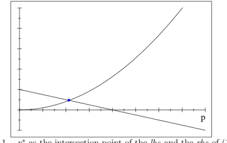
The solution of (13) is the steady-state value of p . Hence, what one intends to investigate is whether there is a solution for this equation and, existing, if it is unique. The lhs of (13) is an increasing and convex function of p that starts at zero (for p = 0); the rhs is a straight line, starting at u > 0 (for p = 0) and with a negative slope. These features force both terms to intersect once and only once for positive values of p . Therefore, a unique p exists
Figure 1 illustrates the steady-state uniqueness for the co-state variable.
p
Fig. 1 - p as the intersection point of the lhs and the rhs of (13).
If a unique p exists, then there will be also just one !i, although this is not necessarily the same across brain systems. Proceeding with the proper computation, one obtains
!i = p =(1 ) A1=(1i ) + p =(1 )X j2N (Aj)1=(1 ) ; i2 N (14)
Note, as well, that the sum of all the resource shares is X j2N !j = p =(1 )X j2N (Aj)1=(1 ) + p =(1 )X j2N (Aj) 1=(1 ) (15)
Expression (15) reveals an important long-term implication of the DAP: as long as parameter assumes a non-zero value, the steady-state result is such that it is optimal for the CES to leave some of the cognitive resources unemployed (this is true because j2N !j < 1). This outcome is the straightforward corollary of costly communication of needs; after a given threshold, the
bene…t of acquiring additional resources for solving tasks does not compensate, on the individual system’s perspective, the costs of convincing the CES to release additional resources.
Next, local stability of the steady-state (!i; pi); i 2 N is evaluated. To proceed, one lin-earizes equations (6)-(7) in the vicinity of the steady-state. The linearization conducts to a 2n dimensional matricial system. The respective Jacobian matrix is conveniently expressed in four blocks, each one corresponding to a square matrix of order n:
J = J11 J12 J21 J22
Matrix Jlm has as elements the derivatives of the state equations (l = 1) / co-state equations (l = 2) with respect to the state variables (m = 1) / co-state variables (m = 2). All the elements are evaluated in the equilibrium position. The following result is determined,
Proposition 4 The linearized system of the DAP is saddle-path stable, with the number of stable trajectories equal to n.
Proof. The number of positive and negative eigenvalues of the Jacobian matrix furnishes the degree of stability underlying the system. To each negative (positive) eigenvalue it corresponds a stable (unstable) dimension. Note that J21 is a matrix of zeros and, therefore, the eigenvalues of J have correspondence on the eigenvalues of J11 and J22. These matrices are,
J11= 2 6 6 6 6 6 6 6 6 6 6 6 6 6 6 6 6 6 6 6 6 4 1 X j2Nnf1g !j 1 X j2N !j !1 1 X j2N !j !1 1 X j2N !j !2 1 X j2N !j 1 X j2Nnf2g !j 1 X j2N !j !2 1 X j2N !j .. . ... . .. ... !n 1 X j2N !j !n 1 X j2N !j 1 X j2Nnfng !j 1 X j2N !j 3 7 7 7 7 7 7 7 7 7 7 7 7 7 7 7 7 7 7 7 7 5 and J22= 2 6 6 6 6 6 6 6 6 6 6 6 6 6 6 6 6 6 6 6 6 4 + 1 X j2Nnf1g !j 1 X j2N !j !2 1 X j2N !j !n 1 X j2N !j !1 1 X j2N !j + 1 X j2Nnf2g !j 1 X j2N !j !n 1 X j2N !j .. . ... . .. ... !1 1 X j2N !j !2 1 X j2N !j + 1 X j2Nnfng !j 1 X j2N !j 3 7 7 7 7 7 7 7 7 7 7 7 7 7 7 7 7 7 7 7 7 5 2185
Eigenvalues of each matrix are straightforward to compute. For J11, "1 = 1 X j2N !j ; "2; :::; "n = For J22, "n+1 = + 1 X j2N !j; "n+2; :::; "2n = +
As it is evident, the n eigenvalues of J11are negative, while the n eigenvalues of J22are positive. Thus, stable and unstable paths are both of dimension n
The stability result guarantees the possibility of convergence from any initial state in the steady-state vicinity to the equilibrium point, since the dimension of the stable path coincides with the number of state variables.
4
Conclusion and Future Work
Evidence from neuroscience indicates that the brain is composed by a multitude of systems of neurons specialized in dealing with di¤erent tasks. Furthermore, cognitive resources are allocated by a central unit that promotes the most e¢ cient conciliation between the available resources and the needs communicated by each system. Therefore, agency relations occur in the brain in a recurrent way. Assuming that the decision-maker is faced with the same tasks period after period, the agency problem can be approached under the form of an optimal control problem.
The laws of motion derived from solving the intertemporal optimization problem deliver some relevant results on the allocation of resources to brain systems. A steady-state exists, it is unique, it is saddle-path stable and it furnishes the long-run optimal allocation of mental resources across tasks. Optimality implies, in this case, that cognitive resources will never be used in their full extent.
As highlighted in Alonso et al. (2014), this type of agency problem is well suited to approach resource allocation in the brain but it does not need to be circumscribed to this; it can also be used to address other issues as, e.g., the optimal allocation of a …nancial budget to the functional areas of a …rm.
Finally, one should note that the undertaken analysis is purely deterministic; the framework might be modi…ed in order to account for the uncertainty that is associated to most of the choices the human mind faces. One way of introducing uncertainty in this model is by considering that the e¢ ciency parameter Ai is a stochastic variable: the matching between communicated needs and resources available to be allocated does not have to be a deterministic process. This observation constitutes a relevant starting point for future work on the theme.
Appendix - First-order Necessary Conditions under
Con-strained Optimization
In this appendix, the reasoning presented in Kamien and Schwartz (1991) respecting bounded controls (section II.10) and state variable inequality constraints (section II.17) is employed to con…rm that equations (9) and (10) represent the necessary conditions for optimality despite the constraints over endogenous variables that are assumed.
Concerning the nonnegativity constraint on the control variables, a complete statement of the necessary optimality condition would be
i(t) = 0 only if @H @ i(t) 0; i2 N i(t) > 0 only if @H @ i(t) = 0; i2 N Since the derivative @@H
i(t) becomes arbitrarily large when i(t) approaches 0, one can exclude the …rst of the above cases and take equation (9) as the relevant optimality condition (and, thus, an optimal solution requires i(t) > 0).
To con…rm that (10) is the other relevant …rst-order condition, one needs to verify that double inequality 0 !i(t) 1 is satis…ed 8 t 2 [0; +1). The …rst inequality requires the nonnegativity of each mental resource share; the second inequality holds for every brain system i if it also holds for the sum of the mental resource shares, X
i2N
!i(t) 1. Let us start by addressing this last condition.
Under the established optimality conditions, the motion of !i(t) is given by (6). The sum of all !i(t) generates the following aggregate constraint,
" X i2N !i(t) # = =(1 )X i2N h A1=(1i )pi(t) =(1 ) i" 1 X i2N !i(t) # X i2N !i(t) (16)
Next, recall that the analysis takes place on the vicinity of the steady-state, i.e., !i(0) is de…ned on the neighborhood of !i, 8i 2 N. The study of the stability in section 3 allowed for the determination of the eigenvalues of the system’s Jacobian matrix. These eigenvalues reveal the qualitative nature of the stability result, in the case, a n-dimensional saddle-path stability outcome, and may also furnish the expressions of each of the stable trajectories; these are,
2 6 6 4 p1(t) p1 p2(t) p2 ::: pn(t) pn 3 7 7 5 = QpQ!1 2 6 6 4 !1(t) !1 !2(t) !2 ::: !n(t) !n 3 7 7 5 (17)
Matrices Qp and Q! are square matrices of order n. The elements of Qp and Q! are the elements of the eigenvectors of the system’s Jacobian matrix that are associated to the negative eigenvalues. Matrix Qp is the sub-matrix of the eigenvectors’ matrix that concerns co-state variables, matrix Q! contains the eigenvectors’elements respecting state variables.
Independently of parameter values, Qp = 0and, therefore, stable trajectories become simply pi(t) = pi;8i 2 N. In section 3, it was revealed that co-state variables have identical values in the steady-state; hence pi(t) = p holds in the convergence to the steady-state. If the value of the co-state variables remains constant as !i(t) converges towards the long-term equilibrium, then only the motion of !i(t) matters. This implies that equation (16) can be represented as
" X i2N !i(t) # = p =(1 )X i2N A1=(1i ) " 1 X i2N !i(t) # X i2N !i(t) (18)
Given steady-state result (15), equation (18) can be simpli…ed, " X i2N !i(t) # = 1 X i2N !i " X i2N !i(t) X i2N !i # (19)
Di¤erential equation (19) has a straightforward solution, X i2N !i(t) = X i2N !i + exp 0 B B @ 1 X i2N !i t 1 C C A " X i2N !i(0) X i2N !i # (20) As long as X i2N !i(0) and X i2N
!i are positive values lower than 1, equation (20) guarantees that the imposed boundaries on X
i2N
!i(t) are never crossed. Variables representing cogni-tive shares will follow stable trajectories such that X
i2N
!i(t) remains, for any t, in the
inter-val X i2N !i(0) X i2N !i(t) X i2N !i for X i2N !i(0) X i2N !i ! or X i2N !i X i2N !i(t) X i2N !i(0) for X i2N !i(0) X i2N !i ! .
To go back to the nonnegativity constraint on each individual !i(t), rewrite equation (6) for a constant p , !i(t) = p =(1 ) A1=(1i ) " 1 X j2N !j(t) # !i(t); i2 N (21)
System (21) is linear and, thus, its solution is
!(t) = ! + Q exp( t)Q 1[!(0) ! ] (22)
with !(t) an order n vector of variables !i(t), !(0) an order n vector of initial values and ! an order n vector of steady-state share values. Matrix is the Jordan matrix of the system (the main diagonal contains the eigenvalues of the respective Jacobian matrix, J11, and the
rest of the elements are zeros), and Q is the corresponding matrix of eigenvectors. Because the eigenvalues in are negative, solution (22) ensures that for every brain system i there is an exponential convergence from !i(0) to !i; if these are both positive, then !i(t) will also be positive for every time period. Obviously, !i(t) are also values lower than 1, as already demonstrated when dealing with the aggregate share equation.
Since the above arguments allow to con…rm that constraint 0 !i(t) 1; 8i 2 N; is compatible with the de…ned law of motion, one does not need to directly incorporate this constraint in the Hamiltonian function and, hence, equation (10) is e¤ectively the relevant optimality condition.
Another important remark to make is that necessary conditions are, in this case, also su¢ -cient conditions for optimality. In Kamien and Schwartz (1991, section II.15), it is stated that if the objective function and the state constraint are both concave in the states and in the controls, and if pi(t) 0, as it is the case, then necessary conditions for optimality are also su¢ cient. This result may fail to hold, however, if corner solutions eventually exist. The above reasoning has made it clear that control variables might be chosen, in conditions of optimality, in order to guarantee i(t) > 0; also, as long as !i(0)is di¤erent from 0 or 1, !i(t)will never fall in one of these two extreme values, since the allocation share variable will follow an exponential trajectory that conducts !i(t) directly to !i 2 (0; 1).
References
[1] Alonso, R.; I. Brocas and J.D. Carrillo (2014). "Resource Allocation in the Brain." Review of Economic Studies 81, 501-534.
[2] Brocas, I. and J.D. Carrillo (2008). "The Brain as a Hierarchical Organization." American Economic Review 98, 1312-1346.
[3] Kamien, M.I. and N.L. Schwartz (1991). Dynamic Optimization - The Calculus of Variations and Optimal Control in Economics and Management, 2nd edition. Bliss, C.J. and M.D. Intriligator (eds.), Advanced Textbooks in Economics 31. Amsterdam: North-Holland.